习题 10.2 - 解答
(a) 表面发散振幅与重整化微扰论的费曼规则
首先分析该理论的表面发散度(Superficial degree of divergence)。在 d=4 维时空下,设图中有 EF 条外源费米子线,EB 条外源标量线。根据拓扑关系 L=PF+PB−V+1 以及顶点条件 2V=2PF+EF 和 V=2PB+EB,可得表面发散度公式为:
D=4L−PF−2PB=4−23EF−EB
我们需要找出所有 D≥0 的振幅:
- EF=0,EB=1⟹D=3 (标量蝌蚪图)。由于拉格朗日量在宇称变换下 ϕ→−ϕ 是不变的,奇数个外源标量场的振幅严格为零。
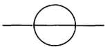
- EF=0,EB=2⟹D=2 (标量场自能),二次发散。
- EF=0,EB=3⟹D=1。由宇称对称性可知该振幅为零。
- EF=0,EB=4⟹D=0 (标量场四点函数),对数发散。
- EF=2,EB=0⟹D=1 (费米子自能),线性发散(实际上由于洛伦兹协变性退化为对数发散)。
- EF=2,EB=1⟹D=0 (汤川顶点),对数发散。
结论与新相互作用:
分析表明,理论中存在一个表面发散的 4ϕ 振幅(EF=0,EB=4)。由于原始拉格朗日量中没有 ϕ4 相互作用项,我们无法用现有的参数来吸收这个发散。因此,必须在原始拉格朗日量中引入标量自相互作用项 δL=4!λϕ4 及其对应的反项,理论才是可重整化的。除此之外,所有其他发散均对应于已有的质量项、动能项或汤川耦合项,不需要引入任何进一步的相互作用。
重整化微扰论的费曼规则:
引入 ϕ4 项后,重整化拉格朗日量(包含反项)写为:
L=21(∂μϕ)2−21m2ϕ2+ψˉ(i∂/−M)ψ−igψˉγ5ψϕ−4!λϕ4+Lct
其中反项拉格朗日量为:
Lct=21δZ(∂μϕ)2−21δmϕ2+ψˉ(iδ2∂/−δM)ψ−iδgψˉγ5ψϕ−4!δλϕ4
对应的费曼规则如下:
- 费米子传播子:p/−M+iϵi
- 标量传播子:p2−m2+iϵi
- 汤川顶点:−igγ5
- ϕ4 顶点:−iλ
- 费米子自能反项:i(p/δ2−δM)
- 标量自能反项:i(p2δZ−δm)
- 汤川顶点反项:−iδgγ5
- ϕ4 顶点反项:−iδλ
(b) 单圈反项的发散部分计算
采用维数正规化 d=4−ϵ。为了提取极点 1/ϵ,可以将外部动量设为最简形式(如 p=0),除非需要提取依赖于外部动量的波函数重整化常数。
1. 费米子自能 (δ2,δM)
单圈费米子自能图为:
−iΣ(p)=∫(2π)dddk(−igγ5)k2−M2i(k/+M)(−igγ5)(p−k)2−m2i
利用 γ5(k/+M)γ5=−k/+M,引入费曼参数 x,令 l=k−xp:
−iΣ(p)=−g2∫01dx∫(2π)dddl(l2−Δ)2−xp/+M
提取发散部分 ∫(2π)dddl(l2−Δ)21→(4π)2iϵ2:
−iΣ(p)div=−g2(4π)2iϵ2∫01dx(−xp/+M)=(4π)2ϵi(g2p/−2g2M)
由抵消条件 i(p/δ2−δM)−iΣ(p)div=0,得到:
δ2=−(4π)2ϵg2,δM=−(4π)2ϵ2g2M
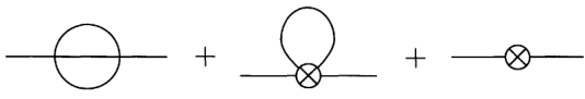
2. 标量场自能 (δZ,δm)
包含费米子圈和标量圈两部分。
费米子圈贡献:
−iΠf(p)=−∫(2π)dddkTr[(−igγ5)k2−M2i(k/+M)(−igγ5)(k+p)2−M2i(k/+p/+M)]
计算迹 Tr[γ5(k/+M)γ5(k/+p/+M)]=−4(k2+k⋅p−M2)。引入费曼参数 x 和 l=k+xp:
−iΠf(p)=4g2∫01dx∫(2π)dddl(l2−Δ)2l2+x(1−x)p2−M2
利用 ∫(2π)dddl(l2−Δ)2l2→(4π)2iϵ4Δ,其中 Δ=M2−x(1−x)p2:
−iΠf(p)div=(4π)24ig2ϵ2∫01dx[2(M2−x(1−x)p2)+x(1−x)p2−M2]=(4π)2ϵ8ig2(M2−61p2)
标量圈贡献(对称因子 1/2):
−iΠs(p)=21(−iλ)∫(2π)dddkk2−m2i→(4π)2ϵiλm2
总发散为 −iΠdiv=(4π)2ϵi[−34g2p2+8g2M2+λm2]。由 i(p2δZ−δm)−iΠdiv=0 得:
δZ=−3(4π)2ϵ4g2,δm=−(4π)2ϵ8g2M2+λm2
3. 汤川顶点 (δg)
单圈顶点图在外部动量为零时的发散部分:
−igΓ5(0,0)=∫(2π)dddk(−igγ5)k2−M2i(k/+M)(−igγ5)k2−M2i(k/+M)(−igγ5)k2−m2i
分子化简:γ5(k/+M)γ5(k/+M)γ5=(−k2+M2)γ5。代入积分:
−igΓ5(0,0)=g3γ5∫(2π)dddk(k2−M2)(k2−m2)1→g3γ5(4π)2iϵ2
由 −iδgγ5−igΓdiv5=0 得:
δg=(4π)2ϵ2g3
4. 标量四点顶点 (δλ)
包含费米子盒图和标量圈图(s, t, u 沟道)。将外部动量设为零。
费米子盒图(共 4!/4=6 个排列):
−iV4f=−6∫(2π)dddkTr[(−igγ5k2−M2i(k/+M))4]
迹的计算:Tr[(γ5(k/+M))4]=Tr[(−k2+M2)2]=4(k2−M2)2。
−iV4f=−6g4∫(2π)dddk(k2−M2)44(k2−M2)2=−24g4∫(2π)dddk(k2−M2)21→−(4π)2ϵ48ig4
标量圈图(3个沟道,每个对称因子 1/2):
−iV4s=3×21(−iλ)2∫(2π)dddkk2−m2ik2−m2i→(4π)2ϵ3iλ2
总发散为 −iVdiv=(4π)2ϵi(3λ2−48g4)。由 −iδλ−iVdiv=0 得:
δλ=(4π)2ϵ3λ2−48g4