The coefficient a2 depends on the details of the renormalization conditions defining αs. Show that the leading two terms in the asymptotic behavior of σ(s) for large s depend only on b0 and b1 and are independent of a2 and b2. Thus the first two coefficients of the QCD β function are independent of the renormalization prescription.
17.2 A direct test of the spin of the gluon. In this problem, we compare the predictions of QCD with those of a model in which the interaction of quarks is mediated by a scalar boson. Let the coupling of the scalar gluon to quarks be given by
δL=gSqˉq,
and define αg=g2/4π.
(a) Using the technique described in parts (b) and (c) of the Final Project of Part I, compute the cross section for e+e−→qqˉS to the leading order of perturbation theory. This cross section depends on the energies of the q, qˉ, and S, which we represent as fractions x1,x2,x3 of the electron beam energy, as in Eq. (17.18). Show that
(b) In practice, it is very difficult to tell quarks from gluons experimentally, since both particles appear as jets of hadrons. Therefore, let xa be the largest of x1,x2,x3, let xb be the second largest, and let xc be the smallest. Sum over the various possibilities to derive an expression for d2σ/dxadxb, both in QCD, using Eq. (17.18), and in the scalar gluon model. Show that these models can be distinguished by their distributions in the xa,xb plane.
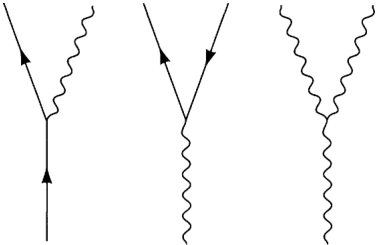
for quark-antiquark annihilation in QCD to the leading order in αs. This is most easily done by computing the amplitudes between states of definite quark and gluon helicity. Ignore all masses. Use explicit polarization vectors and spinors, for example,
ϵμ=21(0,1,i,0)
for a right-handed gluon moving in the +3^ direction. You need only consider transversely polarized gluons. By helicity conservation, only the initial states qLqˉR and qRqˉL can contribute; by parity, these two states give identical cross sections. Thus it is necessary only to compute the amplitudes for the three processes
In fact, by CP invariance, the first and third processes have equal cross sections. After computing the amplitudes, square them and combine them properly with color factors to construct the various helicity cross sections. Finally, combine these to form the total cross section averaged over initial spins and colors.
(b) Compute the differential cross section
dt^dσ(gg→gg)
for gluon-gluon scattering. There are 16 possible combinations of helicities, but many of them are related to each other by parity and crossing symmetry. All 16 can be built up from the three amplitudes for
gRgRgRgRgRgR→gRgR,→gRgL,→gLgL.
Show that the last two of these amplitudes vanish. The first can be dramatically simplified using the Jacobi identity. When the smoke clears, only three of the 16 polarized gluon scattering cross sections are nonzero. Combine these to compute the spin- and color-averaged differential cross section.
17.4 The gluon splitting function. Compute the gluon splitting function (17.130) for the Altarelli-Parisi equations. To carry out this computation, first compute the matrix elements of the three-gluon vertex shown in Fig. 17.20 between gluon states of definite helicity. Combine these to derive the splitting function in the region x<1. Then fix the singularity of the splitting function at x=1 to give this function the correct overall normalization.
17.5 Photoproduction of heavy quarks. Consider the process of heavy quark pair photoproduction, γ+p→QQˉ+X, for a heavy quark of mass M and electric charge Q. If M is large enough, any diagram contributing to this process must involve a large momentum transfer; thus a perturbative QCD analysis should apply. This idea applies in practice already for the production of c quark pairs. Work out the cross section to the leading order in QCD. Choose the parton subprocess that gives the leading contribution to this reaction, and write the parton-model expression for the cross section. You will need to compute the relevant subprocess cross section, but this can be taken directly from one of the QED calculations in Chapter 5. Then use this result to write an expression for the cross section for γ-proton scattering.
17.6 Behavior of parton distribution functions at small x. It is possible to solve the Altarelli-Parisi equations analytically for very small x, using some physically motivated approximations. This discussion is based on a paper of Ralston.†
(a) Show that the Q2 dependence of the right-hand side of the A-P equations can be expressed by rewriting the equations as differential equations in
ξ=loglog(Λ2Q2),
where Λ is the value of Q2 at which αs(Q2), evolved with the leading-order β function, formally goes to infinity.
(b) Since the branching functions to gluons are singular as z−1 as z→0, it is reasonable to guess that the gluon distribution function will blow up approximately as x−1 as x→0. The resulting distribution
dxfg(x)∼xdx
is approximately scale invariant, and so its form should be roughly preserved by the A-P equations. Let us, then, make the following two approximations: (1) the terms involving the gluon distribution completely dominate the right-hand sides of the A-P equations; and (2) the function
g~(x,Q2)=xfg(x,Q2)
is a slowly varying function of x. Using these approximations, and the limit x→0, show that the A-P equation for fg(x) can be converted to the following differential equation:
∂w∂ξ∂2g~(x,ξ)=b012g~(x,ξ),
where w=log(1/x) and b=(11−32nf). Show that if wξ≫1, this equation has the approximate solution
g~=K(Q2)⋅exp([b048w(ξ−ξ0)]1/2),
where K(Q2) is an initial condition.
(c) The quark distribution at very small x is mainly created by branching of gluons. Using the approximations of part (b), show that, for any flavor of quark, the right-hand side of the A-P equation for fq(x) can be approximately integrated to yield an equation for q~(x)=xfq(x):
∂ξ∂q~(x,ξ)=3b02g~(x,ξ).
Show, again using wξ≫1, that this equation has as its integral
with Q02=5 GeV2, Λ=0.2 GeV, and nf=5, gave a reasonable fit to the known properties of parton distributions, extrapolated into the small x region. Use this function and the results above to sketch the behavior of the quark and gluon distributions at small x and large Q2.