20.1 Spontaneous breaking of SU(5). Consider a gauge theory with the gauge group SU(5), coupled to a scalar field Φ in the adjoint representation. Assume that the potential for this scalar field forces it to acquire a nonzero vacuum expectation value. Two possible choices for this expectation value are
⟨Φ⟩=A1111−4and⟨Φ⟩=B222−3−3.
For each case, work out the spectrum of gauge bosons and the unbroken symmetry group.
有质量规范玻色子:对应于混合前三个分量(i∈{1,2,3})与后两个分量(j∈{4,5})的破缺生成元。共有 3×2×2=12 个有质量规范玻色子(即 SU(5) 大统一模型中的 X 和 Y 玻色子)。根据质量公式,它们的质量均为:
M=g∣2B−(−3B)∣=5g∣B∣
20.2
Problem 20.2
peskinChapter 20
习题 20.2
来源: 第20章, PDF第728页
20.2 Decay modes of the W and Z bosons.
(a) Compute the partial decay widths of the W boson into pairs of quarks and leptons. Assume that the top quark mass mt is larger than mW, and ignore the other quark masses. The decay widths to quarks are enhanced by QCD corrections. Show that the correction is given, to order αs, by Eq. (17.9). Using sin2θw=0.23, find a numerical value for the total width of the W+.
(b) Compute the partial decay widths of the Z boson into pairs of quarks and leptons, treating the quarks in the same way as in part (a). Determine the total width of the Z boson and the fractions of the decays that give hadrons, charged leptons, and invisible modes ννˉ.
(a) Consider a fermion species f with electric charge Qf and weak isospin IL3 for its left-handed component. Ignore the mass of the f. Compute the differential cross section for the process e+e−→ffˉ in the standard electroweak model. Include the effect of the Z0 width using the Breit-Wigner formula, Eq. (7.60). Plot the behavior of the total cross section as a function of CM energy through the Z0 resonance, for u, d, and μ.
(b) Compute the forward-backward asymmetry for e+e−→ffˉ, defined as
(c) Show that, just on the Z0 resonance, the forward-backward asymmetry is given by
AFBf=43ALReALRf,
(d) Show that the cross section at the peak of the Z0 resonance is given by
σpeak=mZ212πΓZ2Γ(Z0→e+e−)Γ(Z0→ffˉ),
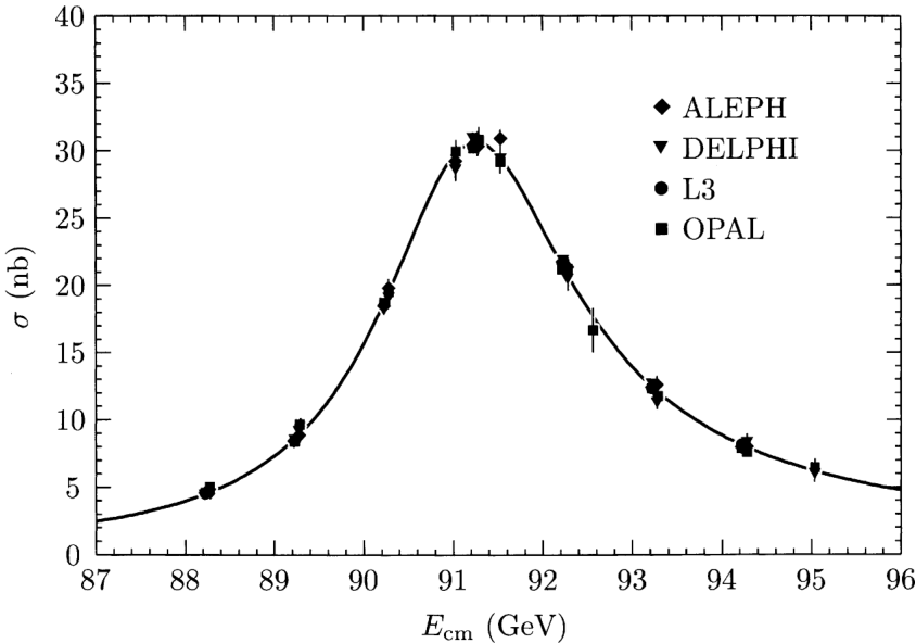
where ΓZ is the total width of the Z0. Notice that both the total width of the Z0 and the peak height are affected by the presence of extra invisible decay modes. Compute the shifts in ΓZ and σpeak that would be produced by a hypothetical fourth neutrino species, and compare these shifts to the cross section measurements shown in Fig. 20.5.
(a) In Eq. (17.35), we wrote formulae for neutrino and antineutrino deep inelastic scattering with W± exchange. Neutrinos and antineutrinos can also scatter by exchanging a Z0. This process, which leads to a hadronic jet but no observable outgoing lepton, is called the neutral current reaction. Compute dσ/dxdy for neutral current deep inelastic scattering of neutrinos and antineutrinos from protons, accounting for scattering from u and d quarks and antiquarks.
(b) Next, consider deep inelastic scattering from a nucleus A with equal numbers of protons and neutrons. For such a target, fu(x)=fd(x), and similarly for antiquarks. Show that the formulae in part (a) simplify in such a situation. In particular, let Rν, Rνˉ be defined as
These formulae remain true when Rν and Rνˉ are redefined to be the ratios of neutral- to charged-current cross sections integrated over the region of x and y that is observed in a given experiment.
(c) By setting r equal to the observed value—say, r=0.4—and varying sin2θw, the relations of part (b) generate a curve in the plane of Rν versus Rνˉ that is known as Weinberg's nose. Sketch this curve. The observed values of Rν,Rνˉ lie close to this curve, near the point corresponding to sin2θw=0.23.
Weinberg’s nose 是一条顶点指向左下方的抛物线,物理点sin2θw=0.23位于最左侧极小值附近。
20.5
Problem 20.5
peskinChapter 20
习题 20.5
来源: 第20章, PDF第729,730页
20.5 A model with two Higgs fields.
(a) Consider a model with two scalar fields ϕ1 and ϕ2, which transform as SU(2) doublets with Y=1/2. Assume that the two fields acquire parallel vacuum expectation values of the form (20.23) with vacuum expectation values v1,v2. Show that these vacuum expectation values produce the same gauge boson mass matrix that we found in Section 20.2, with the replacement
v2→(v12+v22).
(b) The most general potential function for a model with two Higgs doublets is quite complex. However, if we impose the discrete symmetry ϕ1→−ϕ1,ϕ2→ϕ2,
Find conditions on the parameters μi and λi so that the configuration of vacuum expectation values required in part (a) is a locally stable minimum of this potential.
(c) In the unitarity gauge, one linear combination of the upper components of ϕ1 and ϕ2 is eliminated, while the other remains as a physical field. Show that the physical charged Higgs field has the form
ϕ+=sinβϕ1+−cosβϕ2+,
where β is defined by the relation
tanβ=v1v2.
(d) Assume that the two Higgs fields couple to quarks by the set of fundamental couplings
Find the couplings of the physical charged Higgs boson of part (c) to the mass eigenstates of quarks. These couplings depend only on the values of the quark masses and tanβ and on the elements of the CKM matrix.