4.1 Let us return to the problem of the creation of Klein-Gordon particles by a classical source. Recall from Chapter 2 that this process can be described by the Hamiltonian
H=H0+∫d3x(−j(t,x)ϕ(x)),
where H0 is the free Klein-Gordon Hamiltonian, ϕ(x) is the Klein-Gordon field, and j(x) is a c-number scalar function. We found that, if the system is in the vacuum state before the source is turned on, the source will create a mean number of particles
⟨N⟩=∫(2π)3d3p2Ep1∣j~(p)∣2.
In this problem we will verify that statement, and extract more detailed information, by using a perturbation expansion in the strength of the source.
(a) Show that the probability that the source creates no particles is given by
P(0)=⟨0∣T{exp[i∫d4xj(x)ϕI(x)]}∣0⟩2.
(b) Evaluate the term in P(0) of order j2, and show that P(0)=1−λ+O(j4), where λ equals the expression given above for ⟨N⟩.
(c) Represent the term computed in part (b) as a Feynman diagram. Now represent the whole perturbation series for P(0) in terms of Feynman diagrams. Show that this series exponentiates, so that it can be summed exactly: P(0)=exp(−λ).
(d) Compute the probability that the source creates one particle of momentum k. Perform this computation first to O(j) and then to all orders, using the trick of part (c) to sum the series.
(e) Show that the probability of producing n particles is given by
P(n)=(1/n!)λnexp(−λ).
This is a Poisson distribution.
(f) Prove the following facts about the Poisson distribution:
n=0∑∞P(n)=1;⟨N⟩=n=0∑∞nP(n)=λ.
The first identity says that the P(n)'s are properly normalized probabilities, while the second confirms our proposal for ⟨N⟩. Compute the mean square fluctuation ⟨(N−⟨N⟩)2⟩.
4.2 Decay of a scalar particle. Consider the following Lagrangian, involving two real scalar fields Φ and ϕ:
L=21(∂μΦ)2−21M2Φ2+21(∂μϕ)2−21m2ϕ2−μΦϕϕ.
The last term is an interaction that allows a Φ particle to decay into two ϕ's, provided that M>2m. Assuming that this condition is met, calculate the lifetime of the Φ to lowest order in μ.
其中 S 为末态全同粒子的统计对称因子。由于末态是两个相同的 ϕ 粒子,在对全立体角积分时会发生重复计数,故需要除以对称因子 S=2!=2。
将前面求得的物理量代入公式:
Γ=2M1⋅21⋅(4μ2)⋅8π11−M24m2=8πMμ21−M24m2
粒子 Φ 的寿命 τ 是衰变率的倒数:
τ=Γ1=μ21−M24m28πM
最终结果为:
τ=μ21−M24m28πM
4.3
Problem 4.3
peskinChapter 4
习题 4.3
来源: 第4章, PDF第127,128,129页
4.3Linear sigma model. The interactions of pions at low energy can be described by a phenomenological model called the linear sigma model. Essentially, this model consists of N real scalar fields coupled by a ϕ4 interaction that is symmetric under rotations of the N fields. More specifically, let Φi(x), i=1,…,N be a set of N fields, governed by the Hamiltonian
H=∫d3x(21(Πi)2+21(∇Φi)2+V(Φ2)),
where (Φi)2=Φ⋅Φ, and
V(Φ2)=21m2(Φi)2+4λ((Φi)2)2
is a function symmetric under rotations of Φ. For (classical) field configurations of Φi(x) that are constant in space and time, this term gives the only contribution to H; hence, V is the field potential energy.
(What does this Hamiltonian have to do with the strong interactions? There are two types of light quarks, u and d. These quarks have identical strong interactions, but different masses. If these quarks are massless, the Hamiltonian of the strong interactions is invariant to unitary transformations of the 2-component object (u,d):
(ud)→exp(iα⋅σ/2)(ud).
This transformation is called an isospin rotation. If, in addition, the strong interactions are described by a vector "gluon" field (as is true in QCD), the strong interaction Hamiltonian is invariant to the isospin rotations done separately on the left-handed and right-handed components of the quark fields. Thus, the complete symmetry of QCD with two massless quarks is SU(2)×SU(2). It happens that SO(4), the group of rotations in 4 dimensions, is isomorphic to SU(2)×SU(2), so for N=4, the linear sigma model has the same symmetry group as the strong interactions.)
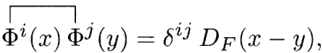
(a) Analyze the linear sigma model for m2>0 by noticing that, for λ=0, the Hamiltonian given above is exactly N copies of the Klein-Gordon Hamiltonian. We can then calculate scattering amplitudes as perturbation series in the parameter λ. Show that the propagator is
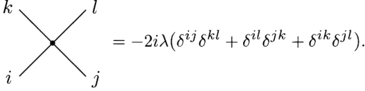
where DF is the standard Klein-Gordon propagator for mass m, and that there is one type of vertex given by
(That is, the vertex between two Φ1s and two Φ2s has the value (−2iλ); that between four Φ1s has the value (−6iλ).) Compute, to leading order in λ, the differential cross sections dσ/dΩ, in the center-of-mass frame, for the scattering processes
Φ1Φ2→Φ1Φ2,Φ1Φ1→Φ2Φ2,andΦ1Φ1→Φ1Φ1
as functions of the center-of-mass energy.
(b) Now consider the case m2<0: m2=−μ2. In this case, V has a local maximum, rather than a minimum, at Φi=0. Since V is a potential energy, this implies that the ground state of the theory is not near Φi=0 but rather is obtained by shifting Φi toward the minimum of V. By rotational invariance, we can consider this shift to be in the Nth direction. Write, then,
Φi(x)ΦN(x)=πi(x),i=1,…,N−1,=v+σ(x),
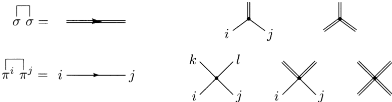
where v is a constant chosen to minimize V. (The notation πi suggests a pion field and should not be confused with a canonical momentum.) Show that, in these new coordinates (and substituting for v its expression in terms of λ and μ), we have a theory of a massive σ field and N−1massless pion fields, interacting through cubic and quartic potential energy terms which all become small as λ→0. Construct the Feynman rules by assigning values to the propagators and vertices:
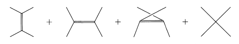
(c) Compute the scattering amplitude for the process
πi(p1)πj(p2)→πk(p3)πl(p4)
to leading order in λ. There are now four Feynman diagrams that contribute:
Show that, at threshold (pi=0), these diagrams sum to zero. (Hint: It may be easiest to first consider the specific process π1π1→π2π2, for which only the first and fourth diagrams are nonzero, before tackling the general case.) Show that, in the special case N=2 (1 species of pion), the term of O(p2) also cancels.
(d) Add to V a symmetry-breaking term,
ΔV=−aΦN,
where a is a (small) constant. (In QCD, a term of this form is produced if the u and d quarks have the same nonvanishing mass.) Find the new value of v that minimizes V, and work out the content of the theory about that point. Show that the pion acquires a mass such that mπ2∼a, and show that the pion scattering amplitude at threshold is now nonvanishing and also proportional to a.
习题 4.3 - 解答
习题 4.3 分析与解答
(a) 对称相 (m2>0) 的线性 σ 模型
1. 传播子与顶点规则
当 λ=0 时,哈密顿量描述了 N 个独立的、质量为 m 的 Klein-Gordon 场。自由场的拉格朗日密度为:
L0=21∂μΦi∂μΦi−21m2ΦiΦi
由于各分量场相互独立,只有同种场的缩并才非零。因此,传播子为:
⟨0∣TΦi(x)Φj(y)∣0⟩=δijDF(x−y)
其中 DF(x−y) 是标准的标量场传播子。
4.4 Rutherford scattering. The cross section for scattering of an electron by the Coulomb field of a nucleus can be computed, to lowest order, without quantizing the electromagnetic field. Instead, treat the field as a given, classical potential Aμ(x). The interaction Hamiltonian is
HI=∫d3xeψˉγμψAμ,
where ψ(x) is the usual quantized Dirac field.
(a) Show that the T-matrix element for electron scattering off a localized classical potential is, to lowest order,
⟨p′∣iT∣p⟩=−ieuˉ(p′)γμu(p)⋅A~μ(p′−p),
where A~μ(q) is the four-dimensional Fourier transform of Aμ(x).
(b) If Aμ(x) is time independent, its Fourier transform contains a delta function of energy. It is then natural to define
⟨p′∣iT∣p⟩≡iM⋅(2π)δ(Ef−Ei),
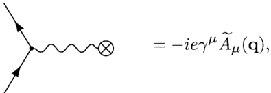
where Ei and Ef are the initial and final energies of the particle, and to adopt a new Feynman rule for computing M:
where A~μ(q) is the three-dimensional Fourier transform of Aμ(x). Given this definition of M, show that the cross section for scattering off a time-independent,
where vi is the particle's initial velocity. This formula is a natural modification of (4.79). Integrate over ∣pf∣ to find a simple expression for dσ/dΩ.
(c) Specialize to the case of electron scattering from a Coulomb potential (A0=Ze/4πr). Working in the nonrelativistic limit, derive the Rutherford formula,
dΩdσ=4m2v4sin4(θ/2)α2Z2.
(With a few calculational tricks from Section 5.1, you will have no difficulty evaluating the general cross section in the relativistic case; see Problem 5.1.)