6.1

Problem 6.1

peskinChapter 6

习题 6.1

来源: 第6章, PDF第208,209页


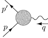
6.1 Rosenbluth formula. As discussed Section 6.2, the exact electromagnetic interaction vertex for a Dirac fermion can be written quite generally in terms of two form factors F1(q2)F_1(q^2) and F2(q2)F_2(q^2):

A Feynman diagram showing a fermion scattering vertex with an incoming fermion p, an outgoing fermion p', and an exchanged photon q, represented by a shaded circle indicating the vertex structure.
=uˉ(p)[γμF1(q2)+iσμνqν2mF2(q2)]u(p),= \bar{u}(p') \left[ \gamma^\mu F_1(q^2) + \frac{i\sigma^{\mu\nu} q_\nu}{2m} F_2(q^2) \right] u(p),

where q=ppq = p' - p and σμν=12i[γμ,γν]\sigma^{\mu\nu} = \frac{1}{2}i[\gamma^\mu, \gamma^\nu]. If the fermion is a strongly interacting particle such as the proton, the form factors reflect the structure that results from the strong interactions and so are not easy to compute from first principles. However, these form factors can be determined experimentally. Consider the scattering of an electron with energy EmeE \gg m_e from a proton initially at rest. Show that the above expression for the vertex leads to the following expression (the Rosenbluth formula) for the elastic scattering cross section, computed to leading order in α\alpha but to all orders in the strong interactions:

dσdcosθ=πα2[(F12q24m2F22)cos2θ2q22m2(F1+F2)2sin2θ2]2E2[1+2Emsin2θ2]sin4θ2,\frac{d\sigma}{d\cos\theta} = \frac{\pi\alpha^2 \left[ (F_1^2 - \frac{q^2}{4m^2} F_2^2) \cos^2 \frac{\theta}{2} - \frac{q^2}{2m^2} (F_1 + F_2)^2 \sin^2 \frac{\theta}{2} \right]}{2E^2 [1 + \frac{2E}{m} \sin^2 \frac{\theta}{2}] \sin^4 \frac{\theta}{2}},

where θ\theta is the lab-frame scattering angle and F1F_1 and F2F_2 are to be evaluated at the q2q^2 associated with elastic scattering at this angle. By measuring (dσ/dcosθ)(d\sigma/d\cos\theta) as a function of angle, it is thus possible to extract F1F_1 and F2F_2. Note that when F1=1F_1 = 1 and F2=0F_2 = 0, the Rosenbluth formula reduces to the Mott formula (in the massless limit) for scattering off a point particle (see Problem 5.1).

习题 6.1 - 解答


物理背景与题目分析

本题要求推导电子-质子弹性散射的 Rosenbluth 公式。在此过程中,电子被视为无质量的点粒子(EmeE \gg m_e),而质子由于强相互作用具有内部结构,其电磁顶点由两个形状因子 F1(q2)F_1(q^2)F2(q2)F_2(q^2) 参数化。 散射过程为 e(k)+p+(p)e(k)+p+(p)e^-(k) + p^+(p) \rightarrow e^-(k') + p^+(p')。 在实验室系中,初始质子静止,运动学变量如下:

  • 初始质子动量:p=(m,0,0,0)p = (m, 0, 0, 0)
  • 初始电子动量:k=(E,0,0,E)k = (E, 0, 0, E)
  • 末态电子动量:k=(E,Esinθ,0,Ecosθ)k' = (E', E'\sin\theta, 0, E'\cos\theta)
  • 动量转移:q=kk=ppq = k - k' = p' - p

首先,我们推导运动学关系。动量转移的平方为: q2=(kk)22kk=2EE(1cosθ)=4EEsin2θ2q^2 = (k - k')^2 \approx -2k \cdot k' = -2EE'(1 - \cos\theta) = -4EE'\sin^2\frac{\theta}{2} 由能量动量守恒 p=p+qp' = p + q,两边平方得 p2=p2+2pq+q2p'^2 = p^2 + 2p \cdot q + q^2。由于质子质量不变 p2=p2=m2p'^2 = p^2 = m^2,我们有: 2pq=q22p \cdot q = -q^2 在实验室系中,pq=m(EE)p \cdot q = m(E - E'),因此: 2m(EE)=4EEsin2θ2    E=E1+2Emsin2θ22m(E - E') = 4EE'\sin^2\frac{\theta}{2} \implies E' = \frac{E}{1 + \frac{2E}{m}\sin^2\frac{\theta}{2}}

解题过程

1. 矩阵元与 Gordon 分解 单光子交换的 Feynman 振幅为: iM=uˉ(k)(ieγμ)u(k)(igμνq2)uˉ(p)[ie(γνF1+iσνρqρ2mF2)]u(p)i\mathcal{M} = \bar{u}(k') (-ie\gamma^\mu) u(k) \left(\frac{-ig_{\mu\nu}}{q^2}\right) \bar{u}(p') \left[ ie \left( \gamma^\nu F_1 + \frac{i\sigma^{\nu\rho}q_\rho}{2m} F_2 \right) \right] u(p) 为了简化后续的迹计算,我们利用 Gordon 恒等式 uˉ(p)γμu(p)=uˉ(p)[(p+p)μ2m+iσμνqν2m]u(p)\bar{u}(p')\gamma^\mu u(p) = \bar{u}(p') \left[ \frac{(p'+p)^\mu}{2m} + \frac{i\sigma^{\mu\nu}q_\nu}{2m} \right] u(p) 重写质子顶点。令 P=p+pP = p + p',则顶点因子可化为: Γμ=γμF1+(γμPμ2m)F2=γμ(F1+F2)Pμ2mF2\Gamma^\mu = \gamma^\mu F_1 + \left( \gamma^\mu - \frac{P^\mu}{2m} \right) F_2 = \gamma^\mu (F_1 + F_2) - \frac{P^\mu}{2m} F_2 于是矩阵元平方的自旋平均为: M2=14spinsM2=e4q4LμνHμν\overline{|\mathcal{M}|^2} = \frac{1}{4} \sum_{\text{spins}} |\mathcal{M}|^2 = \frac{e^4}{q^4} L^{\mu\nu} H_{\mu\nu} 其中电子张量 LμνL^{\mu\nu} 和质子张量 HμνH_{\mu\nu} 分别定义为(包含 1/21/2 因子): Lμν=12Tr[γμ̸ ⁣kγν̸ ⁣k]=2(kμkν+kνkμgμνkk)L^{\mu\nu} = \frac{1}{2} \text{Tr}[\gamma^\mu \slashed{k} \gamma^\nu \slashed{k}'] = 2(k^\mu k'^\nu + k^\nu k'^\mu - g^{\mu\nu} k \cdot k') Hμν=12Tr[Γμ(̸ ⁣p+m)Γˉν(̸ ⁣p+m)]H_{\mu\nu} = \frac{1}{2} \text{Tr}[\Gamma_\mu (\slashed{p} + m) \bar{\Gamma}_\nu (\slashed{p}' + m)]

2. 计算质子张量 HμνH_{\mu\nu}Γμ\Gamma_\mu 代入 HμνH_{\mu\nu} 并展开迹: Hμν=12Tr[(γμ(F1+F2)Pμ2mF2)(̸ ⁣p+m)(γν(F1+F2)Pν2mF2)(̸ ⁣p+m)]H_{\mu\nu} = \frac{1}{2} \text{Tr} \left[ \left( \gamma_\mu (F_1+F_2) - \frac{P_\mu}{2m} F_2 \right) (\slashed{p}+m) \left( \gamma_\nu (F_1+F_2) - \frac{P_\nu}{2m} F_2 \right) (\slashed{p}'+m) \right] 逐项计算迹:

  • γμγν\gamma_\mu \dots \gamma_\nu 项: 12(F1+F2)2Tr[γμ(̸ ⁣p+m)γν(̸ ⁣p+m)]=2(F1+F2)2[pμpν+pνpμgμν(ppm2)]\frac{1}{2} (F_1+F_2)^2 \text{Tr}[\gamma_\mu(\slashed{p}+m)\gamma_\nu(\slashed{p}'+m)] = 2(F_1+F_2)^2 [p_\mu p'_\nu + p_\nu p'_\mu - g_{\mu\nu}(p\cdot p' - m^2)] 利用 ppm2=q2/2p\cdot p' - m^2 = -q^2/2pμpν+pνpμ=12PμPν12qμqνp_\mu p'_\nu + p_\nu p'_\mu = \frac{1}{2}P_\mu P_\nu - \frac{1}{2}q_\mu q_\nu,该项化为: (F1+F2)2[PμPνqμqν+gμνq2](F_1+F_2)^2 [P_\mu P_\nu - q_\mu q_\nu + g_{\mu\nu}q^2]
  • 交叉项: 12(F1+F2)F22mPνTr[γμ(̸ ⁣p+m)(̸ ⁣p+m)]+(μν)-\frac{1}{2} (F_1+F_2) \frac{F_2}{2m} P_\nu \text{Tr}[\gamma_\mu(\slashed{p}+m)(\slashed{p}'+m)] + (\mu \leftrightarrow \nu) 由于 Tr[γμ(̸ ⁣p+m)(̸ ⁣p+m)]=4m(pμ+pμ)=4mPμ\text{Tr}[\gamma_\mu(\slashed{p}+m)(\slashed{p}'+m)] = 4m(p_\mu + p'_\mu) = 4m P_\mu,交叉项总和为: 2(F1+F2)F2PμPν-2(F_1+F_2)F_2 P_\mu P_\nu
  • PμPνP_\mu P_\nu 项: 12F224m2PμPνTr[(̸ ⁣p+m)(̸ ⁣p+m)]=F228m2PμPν4(pp+m2)\frac{1}{2} \frac{F_2^2}{4m^2} P_\mu P_\nu \text{Tr}[(\slashed{p}+m)(\slashed{p}'+m)] = \frac{F_2^2}{8m^2} P_\mu P_\nu \cdot 4(p\cdot p' + m^2) 利用 pp+m2=2m2q2/2p\cdot p' + m^2 = 2m^2 - q^2/2,该项化为: F22(1q24m2)PμPνF_2^2 \left(1 - \frac{q^2}{4m^2}\right) P_\mu P_\nu 将上述三项相加,合并 PμPνP_\mu P_\nu 的系数: (F1+F2)22(F1+F2)F2+F22(1q24m2)=F12q24m2F22(F_1+F_2)^2 - 2(F_1+F_2)F_2 + F_2^2 \left(1 - \frac{q^2}{4m^2}\right) = F_1^2 - \frac{q^2}{4m^2} F_2^2 因此,质子张量简化为: Hμν=(F12q24m2F22)PμPν+(F1+F2)2(gμνq2qμqν)H_{\mu\nu} = \left( F_1^2 - \frac{q^2}{4m^2} F_2^2 \right) P_\mu P_\nu + (F_1+F_2)^2 (g_{\mu\nu} q^2 - q_\mu q_\nu)

3. 张量收缩与矩阵元平方 计算 LμνHμνL^{\mu\nu} H_{\mu\nu}。由于电子无质量,流守恒保证了 qμLμν=0q_\mu L^{\mu\nu} = 0,因此 HμνH_{\mu\nu} 中的 qμqνq_\mu q_\nu 项在收缩时为零。

  • 收缩 PμPνP_\mu P_\nu 项: LμνPμPν=2[2(kP)(kP)P2(kk)]L^{\mu\nu} P_\mu P_\nu = 2[2(k\cdot P)(k'\cdot P) - P^2 (k\cdot k')] 代入运动学关系 kP=2mE+q2/2k\cdot P = 2mE + q^2/2kP=2mEq2/2=2mE+q2/2k'\cdot P = 2mE' - q^2/2 = 2mE + q^2/2P2=4m2q2P^2 = 4m^2 - q^2kk=q2/2k\cdot k' = -q^2/2LμνPμPν=2[2(2mE+q22)2(4m2q2)(q22)]=16m2E2+8mEq2+4m2q2L^{\mu\nu} P_\mu P_\nu = 2 \left[ 2\left(2mE + \frac{q^2}{2}\right)^2 - (4m^2 - q^2)\left(-\frac{q^2}{2}\right) \right] = 16m^2E^2 + 8mEq^2 + 4m^2q^2 利用 q2=2m(EE)q^2 = 2m(E'-E),上式可化简为: 4m2(4E2+2E(EE)+q2/m2m2)=4m2(4EE+q2)4m^2(4E^2 + 2E(E'-E) + q^2/m^2 \cdot m^2) = 4m^2(4EE' + q^2) 代入 q2=4EEsin2θ2q^2 = -4EE'\sin^2\frac{\theta}{2},得到: LμνPμPν=4m2(4EE4EEsin2θ2)=16m2EEcos2θ2L^{\mu\nu} P_\mu P_\nu = 4m^2 \left( 4EE' - 4EE'\sin^2\frac{\theta}{2} \right) = 16m^2 EE' \cos^2\frac{\theta}{2}
  • 收缩 gμνq2g_{\mu\nu} q^2 项: Lμνgμνq2=q2Lμμ=q22(2kk4kk)=4q2(kk)=2q4L^{\mu\nu} g_{\mu\nu} q^2 = q^2 L^\mu_\mu = q^2 \cdot 2(2k\cdot k' - 4k\cdot k') = -4q^2 (k\cdot k') = 2q^4 代入 q2=4EEsin2θ2q^2 = -4EE'\sin^2\frac{\theta}{2},得到: 2q4=2q2(4EEsin2θ2)=8EEq2sin2θ22q^4 = 2q^2 \left( -4EE'\sin^2\frac{\theta}{2} \right) = -8EE' q^2 \sin^2\frac{\theta}{2} 将两部分组合,得到矩阵元平方: M2=e4q4[16m2EEcos2θ2(F12q24m2F22)8EEq2sin2θ2(F1+F2)2]\overline{|\mathcal{M}|^2} = \frac{e^4}{q^4} \left[ 16m^2 EE' \cos^2\frac{\theta}{2} \left( F_1^2 - \frac{q^2}{4m^2} F_2^2 \right) - 8EE' q^2 \sin^2\frac{\theta}{2} (F_1+F_2)^2 \right] 提取公因子 16e4m2EEq4\frac{16e^4 m^2 EE'}{q^4}M2=16e4m2EEq4[(F12q24m2F22)cos2θ2q22m2(F1+F2)2sin2θ2]\overline{|\mathcal{M}|^2} = \frac{16e^4 m^2 EE'}{q^4} \left[ \left( F_1^2 - \frac{q^2}{4m^2} F_2^2 \right) \cos^2\frac{\theta}{2} - \frac{q^2}{2m^2} (F_1+F_2)^2 \sin^2\frac{\theta}{2} \right]

4. 计算微分截面 实验室系中 1+23+41+2 \rightarrow 3+4 散射的微分截面公式为: dσ=14mEd3k(2π)32Ed3p(2π)32Ep(2π)4δ(4)(k+pkp)M2d\sigma = \frac{1}{4mE} \int \frac{d^3 k'}{(2\pi)^3 2E'} \frac{d^3 p'}{(2\pi)^3 2E_p'} (2\pi)^4 \delta^{(4)}(k+p-k'-p') \overline{|\mathcal{M}|^2} 完成对 d3pd^3 p'EE' 的相空间积分,得到: dσdΩ=164π2m2(EE)2M2\frac{d\sigma}{d\Omega} = \frac{1}{64\pi^2 m^2} \left(\frac{E'}{E}\right)^2 \overline{|\mathcal{M}|^2}M2\overline{|\mathcal{M}|^2} 代入,并利用 q4=16E2E2sin4θ2q^4 = 16E^2 E'^2 \sin^4\frac{\theta}{2}dσdΩ=E264π2m2E216e4m2EE16E2E2sin4θ2[]=e4E64π2E3sin4θ2[]\frac{d\sigma}{d\Omega} = \frac{E'^2}{64\pi^2 m^2 E^2} \frac{16e^4 m^2 EE'}{16E^2 E'^2 \sin^4\frac{\theta}{2}} \left[ \dots \right] = \frac{e^4 E'}{64\pi^2 E^3 \sin^4\frac{\theta}{2}} \left[ \dots \right] 使用精细结构常数 α=e24π\alpha = \frac{e^2}{4\pi},即 e4=16π2α2e^4 = 16\pi^2 \alpha^2dσdΩ=α2E4E3sin4θ2[]\frac{d\sigma}{d\Omega} = \frac{\alpha^2 E'}{4 E^3 \sin^4\frac{\theta}{2}} \left[ \dots \right] 代入 E=E1+2Emsin2θ2E' = \frac{E}{1 + \frac{2E}{m}\sin^2\frac{\theta}{2}},并利用 dΩ=2πd(cosθ)d\Omega = 2\pi d(\cos\theta) 转换为对 cosθ\cos\theta 的微商: dσdcosθ=2πdσdΩ=πα22E2(1+2Emsin2θ2)sin4θ2[]\frac{d\sigma}{d\cos\theta} = 2\pi \frac{d\sigma}{d\Omega} = \frac{\pi \alpha^2}{2 E^2 \left(1 + \frac{2E}{m}\sin^2\frac{\theta}{2}\right) \sin^4\frac{\theta}{2}} \left[ \dots \right] 将方括号中的项完整写出,即得到最终的 Rosenbluth 公式:

dσdcosθ=πα2[(F12q24m2F22)cos2θ2q22m2(F1+F2)2sin2θ2]2E2[1+2Emsin2θ2]sin4θ2\boxed{ \frac{d\sigma}{d\cos\theta} = \frac{\pi\alpha^2 \left[ \left(F_1^2 - \frac{q^2}{4m^2} F_2^2\right) \cos^2 \frac{\theta}{2} - \frac{q^2}{2m^2} (F_1 + F_2)^2 \sin^2 \frac{\theta}{2} \right]}{2E^2 \left[1 + \frac{2E}{m} \sin^2 \frac{\theta}{2}\right] \sin^4 \frac{\theta}{2}} }
6.2

Problem 6.2

peskinChapter 6

习题 6.2

来源: 第6章, PDF第209,210页


6.2 Equivalent photon approximation. Consider the process in which electrons of very high energy scatter from a target. In leading order in α\alpha, the electron is connected to the target by one photon propagator. If the initial and final energies of the electron are EE and EE', the photon will carry momentum qq such that q22EE(1cosθ)q^2 \approx -2EE'(1 - \cos\theta). In the limit of forward scattering, whatever the energy loss, the photon momentum approaches q2=0q^2 = 0; thus the reaction is highly peaked in the forward direction. It is tempting to guess that, in this limit, the virtual photon becomes a real photon. Let us investigate in what sense that is true.

(a) The matrix element for the scattering process can be written as

M=(ie)uˉ(p)γμu(p)igμνq2M^ν(q),\mathcal{M} = (-ie)\bar{u}(p')\gamma^\mu u(p) \frac{-ig_{\mu\nu}}{q^2} \widehat{\mathcal{M}}^\nu(q),

where M^ν\widehat{\mathcal{M}}^\nu represents the (in general, complicated) coupling of the virtual photon to the target. Let us analyze the structure of the piece uˉ(p)γμu(p)\bar{u}(p')\gamma^\mu u(p). Let q=(q0,q)q = (q^0, \mathbf{q}), and define q~=(q0,q)\tilde{q} = (q^0, -\mathbf{q}). We can expand the spinor product as:

uˉ(p)γμu(p)=Aqμ+Bq~μ+Cϵ1μ+Dϵ2μ,\bar{u}(p')\gamma^\mu u(p) = A \cdot q^\mu + B \cdot \tilde{q}^\mu + C \cdot \epsilon_1^\mu + D \cdot \epsilon_2^\mu,

where A,B,C,DA, B, C, D are functions of the scattering angle and energy loss and ϵi\epsilon_i are two unit vectors transverse to q\mathbf{q}. By dotting this expression with qμq_\mu, show that the coefficient BB is at most of order θ2\theta^2. This will mean that we can ignore it in the rest of the analysis. The coefficient AA is large, but it is also irrelevant, since, by the Ward identity, qμM^μ=0q^\mu \widehat{\mathcal{M}}_\mu = 0.

(b) Working in the frame where p=(E,0,0,E)p = (E, 0, 0, E), compute explicitly

uˉ(p)γϵiu(p)\bar{u}(p')\gamma \cdot \epsilon_i u(p)

using massless electrons, u(p)u(p) and u(p)u(p') spinors of definite helicity, and ϵ1,ϵ2\epsilon_1, \epsilon_2 unit vectors parallel and perpendicular to the plane of scattering. We need this quantity only for scattering near the forward direction, and we need only the term of order θ\theta. Note, however, that for ϵ\epsilon in the plane of scattering, the small 3^\hat{3} component of ϵ\epsilon also gives a term of order θ\theta which must be taken into account.

(c) Now write the expression for the electron scattering cross section, in terms of Mμ2|\mathcal{M}^\mu|^2 and the integral over phase space on the target side. This expression must be integrated over the final electron momentum pp'. The integral over p3p'^3 is an integral over the energy loss of the electron. Show that the integral over pp'_\perp diverges logarithmically as pp'_\perp or θ0\theta \rightarrow 0.

(d) The divergence as θ0\theta \rightarrow 0 appears because we have ignored the electron mass in too many places. Show that reintroducing the electron mass in the expression for q2q^2,

q2=2(EEppcosθ)+2m2,q^2 = -2(EE' - pp' \cos\theta) + 2m^2,

cuts off the divergence and yields a factor of log(s/m2)\log(s/m^2) in its place.

(e) Assembling all the factors, and assuming that the target cross sections are independent of the photon polarization, show that the largest part of the electron-target scattering cross section is given by considering the electron to be the source of a beam of real photons with energy distribution (x=Eγ/Ex = E_{\gamma}/E):

Nγ(x)dx=dxxα2π[1+(1x)2]log(sm2).N_{\gamma}(x)dx = \frac{dx}{x} \frac{\alpha}{2\pi} [1 + (1 - x)^2] \log\left(\frac{s}{m^2}\right).

This is the Weizsäcker-Williams equivalent photon approximation. This phenomenon allows us, for example, to study photon-photon scattering using e+ee^+e^- collisions. Notice that the distribution we have found here is the same one that appeared in Problem 5.5 when we considered soft photon emission before electron scattering. It should be clear that a parallel general derivation can be constructed for that case.

习题 6.2 - 解答


(a) 矩阵元结构与系数 BB 的分析

在极高能近似下,电子的初末态动量分别为 pppp',传递的动量为 q=ppq = p - p'。根据狄拉克方程,旋量满足 ̸ ⁣pu(p)=mu(p)\slashed{p}u(p) = m u(p)uˉ(p)̸ ⁣p=muˉ(p)\bar{u}(p')\slashed{p'} = m \bar{u}(p')。 将展开式 uˉ(p)γμu(p)=Aqμ+Bq~μ+Cϵ1μ+Dϵ2μ\bar{u}(p')\gamma^\mu u(p) = A q^\mu + B \tilde{q}^\mu + C \epsilon_1^\mu + D \epsilon_2^\mu 两边同乘 qμq_\mu

qμuˉ(p)γμu(p)=uˉ(p)̸ ⁣qu(p)=uˉ(p)(̸ ⁣p̸ ⁣p)u(p)=0q_\mu \bar{u}(p')\gamma^\mu u(p) = \bar{u}(p')\slashed{q} u(p) = \bar{u}(p')(\slashed{p} - \slashed{p'}) u(p) = 0

由于 ϵ1\epsilon_1ϵ2\epsilon_2 是垂直于 q\mathbf{q} 的单位向量,且 q0=q~0,q=q~q^0 = \tilde{q}^0, \mathbf{q} = -\tilde{\mathbf{q}},我们有 qϵi=0q \cdot \epsilon_i = 0。因此等式右边变为:

Aq2+B(qq~)=0    B=Aq2qq~A q^2 + B (q \cdot \tilde{q}) = 0 \implies B = -A \frac{q^2}{q \cdot \tilde{q}}

在小角散射极限下,能量 Ep,EpE \approx p, E' \approx p',动量传递的平方为:

q22EE(1cosθ)EEθ2q^2 \approx -2EE'(1 - \cos\theta) \approx -EE'\theta^2

qq~q \cdot \tilde{q} 为:

qq~=(q0)2qq~=(q0)2+q2(EE)2+(EE)2=2(EE)2q \cdot \tilde{q} = (q^0)^2 - \mathbf{q} \cdot \tilde{\mathbf{q}} = (q^0)^2 + |\mathbf{q}|^2 \approx (E-E')^2 + (E-E')^2 = 2(E-E')^2

因此,系数 BB 的量级为:

BAEEθ22(EE)2O(θ2)B \approx A \frac{EE'\theta^2}{2(E-E')^2} \sim \mathcal{O}(\theta^2)

这表明 BB 最多是 θ2\theta^2 阶的,在小角前向散射极限下可以忽略。

(b) 极化向量与矩阵元的显式计算

p=(E,0,0,E)p = (E, 0, 0, E) 的参考系中,末态动量为 p=(E,Esinθ,0,Ecosθ)p' = (E', E'\sin\theta, 0, E'\cos\theta)。 光子动量 q=pp(xE,Eθ,0,xE)q = p - p' \approx (xE, -E'\theta, 0, xE),其中 x=(EE)/Ex = (E-E')/E。 取垂直于散射平面的极化向量 ϵ2=(0,0,1,0)\epsilon_2 = (0, 0, 1, 0)。平行于散射平面且正交于 qq 的极化向量 ϵ1\epsilon_1 满足 qϵ1=0q \cdot \epsilon_1 = 0,归一化后在小 θ\theta 极限下为:

ϵ1(0,1,0,EθxE)\epsilon_1 \approx \left(0, 1, 0, \frac{E'\theta}{xE}\right)

对于无质量电子,螺旋度守恒。取右旋旋量(Weyl基底):

uR(p)=2E(0010),uR(p)2E(001θ/2)u_R(p) = \sqrt{2E} \begin{pmatrix} 0 \\ 0 \\ 1 \\ 0 \end{pmatrix}, \quad u_R(p') \approx \sqrt{2E'} \begin{pmatrix} 0 \\ 0 \\ 1 \\ \theta/2 \end{pmatrix}

计算矩阵元 uˉR(p)γμuR(p)=4EE(1,θ/2)σμ(1,0)T\bar{u}_R(p') \gamma^\mu u_R(p) = \sqrt{4EE'} (1, \theta/2) \sigma^\mu (1, 0)^T: 对于 ϵ1\epsilon_1,有 ϵ1γ=γ1EθxEγ3\epsilon_1 \cdot \gamma = -\gamma^1 - \frac{E'\theta}{xE}\gamma^3

uˉR(p)γϵ1uR(p)=4EE(θ2+EθxE)=EEθ(1+2(1x)x)=EEθ2xx\bar{u}_R(p') \gamma \cdot \epsilon_1 u_R(p) = -\sqrt{4EE'} \left( \frac{\theta}{2} + \frac{E'\theta}{xE} \right) = -\sqrt{EE'}\theta \left( 1 + \frac{2(1-x)}{x} \right) = -\sqrt{EE'}\theta \frac{2-x}{x}

对于 ϵ2\epsilon_2,有 ϵ2γ=γ2\epsilon_2 \cdot \gamma = -\gamma^2

uˉR(p)γϵ2uR(p)=4EE(iθ2)=iEEθ\bar{u}_R(p') \gamma \cdot \epsilon_2 u_R(p) = -\sqrt{4EE'} \left( i\frac{\theta}{2} \right) = -i\sqrt{EE'}\theta

左旋电子的结果仅在 ϵ2\epsilon_2 处差一个符号。因此系数 CCDD 的模方和为:

C2+D2=EEθ2[(2xx)2+1]=2EEθ21+(1x)2x2|C|^2 + |D|^2 = EE'\theta^2 \left[ \left(\frac{2-x}{x}\right)^2 + 1 \right] = 2EE'\theta^2 \frac{1+(1-x)^2}{x^2}

(c) 电子散射截面与对数发散

电子-靶散射的微分散射截面为:

dσ=12sd3p(2π)32Ee2(q2)2(C2+D2)dΠtargetM^1 pol2d\sigma = \frac{1}{2s} \frac{d^3p'}{(2\pi)^3 2E'} \frac{e^2}{(q^2)^2} \left( |C|^2 + |D|^2 \right) \int d\Pi_{\text{target}} |\widehat{\mathcal{M}}_{\text{1 pol}}|^2

真实光子-靶的散射截面 σγ(xE)\sigma_\gamma(xE) 满足:

dΠtargetM^1 pol2=2(xs)σγ(xE)\int d\Pi_{\text{target}} |\widehat{\mathcal{M}}_{\text{1 pol}}|^2 = 2(xs) \sigma_\gamma(xE)

相空间元 d3p2πE2dEθdθ=2πdEpdpd^3p' \approx 2\pi E'^2 dE' \theta d\theta = 2\pi dE' p'_\perp dp'_\perp,且 q2EEθ2=Ep2/Eq^2 \approx -EE'\theta^2 = -E p'^2_\perp / E'。代入截面公式:

dσ=12s2πdEpdp16π3E4πα(Ep2/E)2(2EEp21+(1x)2x2)2xsσγd\sigma = \frac{1}{2s} \frac{2\pi dE' p'_\perp dp'_\perp}{16\pi^3 E'} \frac{4\pi\alpha}{(E p'^2_\perp / E')^2} \left( 2 \frac{E}{E'} p'^2_\perp \frac{1+(1-x)^2}{x^2} \right) 2xs \sigma_\gamma

化简并利用 dE=EdxdE' = E dx

dσ=απdxdpp1+(1x)2xσγ(xE)d\sigma = \frac{\alpha}{\pi} dx \frac{dp'_\perp}{p'_\perp} \frac{1+(1-x)^2}{x} \sigma_\gamma(xE)

pp'_\perp 的积分 dpp\int \frac{dp'_\perp}{p'_\perp}p0p'_\perp \to 0(即 θ0\theta \to 0)时呈现对数发散。

(d) 引入电子质量截断发散

恢复电子质量 mm,动量大小 pEm2/(2E)p \approx E - m^2/(2E),此时 q2q^2 变为:

q2=2(EEppcosθ)+2m2EEθ2m2(EE+EE2)=EEθ2m2x21xq^2 = -2(EE' - pp'\cos\theta) + 2m^2 \approx -EE'\theta^2 - m^2\left(\frac{E}{E'} + \frac{E'}{E} - 2\right) = -EE'\theta^2 - m^2\frac{x^2}{1-x}

截面中关于 θ\theta 的积分变为:

θ3dθ(EEθ2+m2x21x)2=12(EE)20E2ydy(y+m2x21x)212(EE)2log(sm2)\int \frac{\theta^3 d\theta}{(EE'\theta^2 + m^2 \frac{x^2}{1-x})^2} = \frac{1}{2(EE')^2} \int_0^{\sim E^2} \frac{y dy}{(y + m^2 \frac{x^2}{1-x})^2} \approx \frac{1}{2(EE')^2} \log\left(\frac{s}{m^2}\right)

这消除了 θ0\theta \to 0 的发散,并将原本的 dpp\int \frac{dp'_\perp}{p'_\perp} 替换为了 12log(sm2)\frac{1}{2}\log\left(\frac{s}{m^2}\right)

(e) 等效光子近似 (Weizsäcker-Williams Approximation)

将 (d) 中的积分结果代入 (c) 的截面表达式中,原本的 dpp\int \frac{dp'_\perp}{p'_\perp} 贡献了因子 12log(sm2)\frac{1}{2}\log\left(\frac{s}{m^2}\right),我们得到:

dσ=[α2πdx1+(1x)2xlog(sm2)]σγ(xE)d\sigma = \left[ \frac{\alpha}{2\pi} dx \frac{1+(1-x)^2}{x} \log\left(\frac{s}{m^2}\right) \right] \sigma_\gamma(xE)

这表明电子-靶的散射截面可以分解为等效真实光子通量 Nγ(x)dxN_\gamma(x)dx 与光子-靶散射截面 σγ\sigma_\gamma 的乘积,其中等效光子分布为:

Nγ(x)dx=dxxα2π[1+(1x)2]log(sm2)\boxed{ N_\gamma(x)dx = \frac{dx}{x} \frac{\alpha}{2\pi} [1 + (1 - x)^2] \log\left(\frac{s}{m^2}\right) }
6.3

Problem 6.3

peskinChapter 6

习题 6.3

来源: 第6章, PDF第210页


6.3 Exotic contributions to g2g - 2. Any particle that couples to the electron can produce a correction to the electron-photon form factors and, in particular, a correction to g2g - 2. Because the electron g2g - 2 agrees with QED to high accuracy, these corrections allow us to constrain the properties of hypothetical new particles.

(a) The unified theory of weak and electromagnetic interactions contains a scalar particle hh called the Higgs boson, which couples to the electron according to

Hint=d3xλ2hψˉψ.H_{\text{int}} = \int d^3x \frac{\lambda}{\sqrt{2}} h \bar{\psi}\psi.

Compute the contribution of a virtual Higgs boson to the electron (g2g - 2), in terms of λ\lambda and the mass mhm_h of the Higgs boson.

(b) QED accounts extremely well for the electron's anomalous magnetic moment. If a=(g2)/2a = (g - 2)/2,

aexpt.aQED<1×10¹⁰.|a_{\text{expt.}} - a_{\text{QED}}| < 1 \times 10^{-10}.

What limits does this place on λ\lambda and mhm_h? In the simplest version of the electroweak theory, λ=3×10⁶\lambda = 3 \times 10^{-6} and mh>60 GeVm_h > 60\text{ GeV}. Show that these values are not excluded. The coupling of the Higgs boson to the muon is larger by a factor (mμ/me)(m_{\mu}/m_e): λ=6×10⁴\lambda = 6 \times 10^{-4}. Thus, although our experimental knowledge of the muon anomalous magnetic moment is not as precise,

aexpt.aQED<3×10⁸,|a_{\text{expt.}} - a_{\text{QED}}| < 3 \times 10^{-8},

one can still obtain a stronger limit on mhm_h. Is it strong enough?

(c) Some more complex versions of this theory contain a pseudoscalar particle called the axion, which couples to the electron according to

Hint=d3xiλ2aψˉγ5ψ.H_{\text{int}} = \int d^3x \frac{i\lambda}{\sqrt{2}} a \bar{\psi}\gamma^5\psi.

The axion may be as light as the electron, or lighter, and may couple more strongly than the Higgs boson. Compute the contribution of a virtual axion to the g2g - 2 of the electron, and work out the excluded values of λ\lambda and mam_a.

习题 6.3 - 解答


(a) 虚拟 Higgs 玻色子对电子 (g2)(g-2) 的贡献

相互作用哈密顿量为 Hint=d3xλ2hψˉψH_{\text{int}} = \int d^3x \frac{\lambda}{\sqrt{2}} h \bar{\psi}\psi,对应的顶点 Feynman 规则为 iλ2-i\frac{\lambda}{\sqrt{2}}。 我们计算包含虚拟 Higgs 玻色子 hh 的单圈顶点修正。设入射电子动量为 pp,出射电子动量为 pp',光子动量为 q=ppq = p' - p。单圈顶点函数 ieΓμ(p,p)-ie\Gamma^\mu(p', p) 为: ieΓμ=d4k(2π)4(iλ2)i(̸ ⁣p̸ ⁣k+m)(pk)2m2(ieγμ)i(̸ ⁣p̸ ⁣k+m)(pk)2m2(iλ2)ik2mh2-ie\Gamma^\mu = \int \frac{d^4k}{(2\pi)^4} \left(-i\frac{\lambda}{\sqrt{2}}\right) \frac{i(\slashed{p}' - \slashed{k} + m)}{(p'-k)^2 - m^2} (-ie\gamma^\mu) \frac{i(\slashed{p} - \slashed{k} + m)}{(p-k)^2 - m^2} \left(-i\frac{\lambda}{\sqrt{2}}\right) \frac{i}{k^2 - m_h^2} 化简常数因子,并引入 Feynman 参数 x,y,zx, y, z(满足 x+y+z=1x+y+z=1): Γμ=iλ22dxdydzδ(x+y+z1)d4k(2π)42NhμD3\Gamma^\mu = -i\frac{\lambda^2}{2} \int dxdydz \delta(x+y+z-1) \int \frac{d^4k}{(2\pi)^4} \frac{2 N^\mu_h}{D^3} 其中分母 D=x((pk)2m2)+y((pk)2m2)+z(k2mh2)D = x((p'-k)^2 - m^2) + y((p-k)^2 - m^2) + z(k^2 - m_h^2)。 配方并平移积分变量 l=k(xp+yp)l = k - (xp' + yp),在 q20q^2 \to 0 的极限下(由对称性 x=y=(1z)/2x=y=(1-z)/2),分母变为 D=l2ΔhD = l^2 - \Delta_h,其中 Δh=(1z)2m2+zmh2\Delta_h = (1-z)^2 m^2 + z m_h^2

分子部分为 Nhμ=(̸ ⁣p̸ ⁣k+m)γμ(̸ ⁣p̸ ⁣k+m)N^\mu_h = (\slashed{p}' - \slashed{k} + m) \gamma^\mu (\slashed{p} - \slashed{k} + m)。 由于我们只关心夹在旋量 uˉ(p)\bar{u}(p')u(p)u(p) 之间的矩阵元,可以利用 Dirac 方程 uˉ(p)̸ ⁣p=muˉ(p)\bar{u}(p')\slashed{p}' = m\bar{u}(p')̸ ⁣pu(p)=mu(p)\slashed{p}u(p) = m u(p),将分子等效替换为: Nhμ(2m̸ ⁣k)γμ(2m̸ ⁣k)=4m2γμ4mkμ+̸ ⁣kγμ̸ ⁣kN^\mu_h \doteq (2m - \slashed{k}) \gamma^\mu (2m - \slashed{k}) = 4m^2 \gamma^\mu - 4m k^\mu + \slashed{k} \gamma^\mu \slashed{k} 利用 ̸ ⁣kγμ̸ ⁣k=2kμ̸ ⁣kk2γμ\slashed{k} \gamma^\mu \slashed{k} = 2k^\mu \slashed{k} - k^2 \gamma^\mu,并代入 k=l+xp+ypk = l + xp' + yp。奇数阶 ll 的项积分后为零,而正比于 γμ\gamma^\mu 的项只对电荷形状因子 F1F_1 有贡献,不贡献反常磁矩 F2F_2。 我们只需提取出正比于 iσμνqνi\sigma^{\mu\nu}q_\nu 的项。利用 Gordon 恒等式 (p+p)μ=2mγμ+iσμνqν(p+p')^\mu = 2m\gamma^\mu + i\sigma^{\mu\nu}q_\nu,我们有: kμ1z2(p+p)μ=1z2(2mγμ+iσμνqν)k^\mu \doteq \frac{1-z}{2}(p+p')^\mu = \frac{1-z}{2}(2m\gamma^\mu + i\sigma^{\mu\nu}q_\nu) 2kμ̸ ⁣k21z2(p+p)μ(1z)m=m(1z)2(2mγμ+iσμνqν)2k^\mu \slashed{k} \doteq 2 \frac{1-z}{2}(p+p')^\mu (1-z)m = m(1-z)^2 (2m\gamma^\mu + i\sigma^{\mu\nu}q_\nu) 因此,NhμN^\mu_h 中包含 iσμνqνi\sigma^{\mu\nu}q_\nu 的系数为: 4m(1z2)+m(1z)2=m(1z)(1+z)=m(1z2)-4m \left(\frac{1-z}{2}\right) + m(1-z)^2 = -m(1-z)(1+z) = -m(1-z^2) 根据定义 Γμ=γμF1+iσμνqν2mF2\Gamma^\mu = \gamma^\mu F_1 + \frac{i\sigma^{\mu\nu}q_\nu}{2m} F_2,我们得到 F2F_2 的被积函数部分为 2m×[m(1z2)]=2m2(1z2)2m \times [-m(1-z^2)] = -2m^2(1-z^2)。 完成动量 ll 的积分 d4l(2π)41(l2Δh)3=i32π2Δh\int \frac{d^4l}{(2\pi)^4} \frac{1}{(l^2 - \Delta_h)^3} = \frac{-i}{32\pi^2 \Delta_h},得到 Higgs 玻色子对电子反常磁矩的贡献 ah=F2(0)a_h = F_2(0)ah=iλ2201dz(1z)2i32π2Δh[2m2(1z2)]=λ2m216π201dz(1z)2(1+z)(1z)2m2+zmh2a_h = -i\frac{\lambda^2}{2} \int_0^1 dz (1-z) \frac{-2i}{32\pi^2 \Delta_h} [-2m^2(1-z^2)] = \frac{\lambda^2 m^2}{16\pi^2} \int_0^1 dz \frac{(1-z)^2(1+z)}{(1-z)^2 m^2 + z m_h^2} 最终结果为: ah=λ2me216π201dz(1z)2(1+z)(1z)2me2+zmh2\boxed{ a_h = \frac{\lambda^2 m_e^2}{16\pi^2} \int_0^1 dz \frac{(1-z)^2(1+z)}{(1-z)^2 m_e^2 + z m_h^2} }

(b) 对 λ\lambdamhm_h 的限制

对于电子,已知 memhm_e \ll m_h,积分主要由 z0z \to 0 区域贡献,近似为: ahλ2me216π2mh201dzz+(me/mh)2λ2me28π2mh2ln(mhme)a_h \approx \frac{\lambda^2 m_e^2}{16\pi^2 m_h^2} \int_0^1 \frac{dz}{z + (m_e/m_h)^2} \approx \frac{\lambda^2 m_e^2}{8\pi^2 m_h^2} \ln\left(\frac{m_h}{m_e}\right) 代入 λ=3×10⁶\lambda = 3 \times 10^{-6}mh=60 GeVm_h = 60\text{ GeV}me=0.511 MeVm_e = 0.511\text{ MeV}ah(3×10⁶)28π2(0.511×10360)2ln(600.511×10³)1.2×10²²a_h \approx \frac{(3 \times 10^{-6})^2}{8\pi^2} \left(\frac{0.511 \times 10^{-3}}{60}\right)^2 \ln\left(\frac{60}{0.511 \times 10^{-3}}\right) \approx 1.2 \times 10^{-22} 这远小于实验误差界限 1×10101 \times 10^{-10},因此 这些值未被排除

对于 μ\mu 子,λ=6×10⁴\lambda = 6 \times 10^{-4}mμ=105.6 MeVm_\mu = 105.6\text{ MeV}ah(μ)(6×10⁴)28π2(0.10660)2ln(600.106)9×10¹⁴a_h^{(\mu)} \approx \frac{(6 \times 10^{-4})^2}{8\pi^2} \left(\frac{0.106}{60}\right)^2 \ln\left(\frac{60}{0.106}\right) \approx 9 \times 10^{-14} 这依然远小于 μ\mu 子的实验误差界限 3×1083 \times 10^{-8}。 事实上,要求 ah(μ)<3×10⁸a_h^{(\mu)} < 3 \times 10^{-8} 给出: mμ2mh2ln(mhmμ)<8π2×3×108(6×10⁴)26.6\frac{m_\mu^2}{m_h^2} \ln\left(\frac{m_h}{m_\mu}\right) < \frac{8\pi^2 \times 3 \times 10^{-8}}{(6 \times 10^{-4})^2} \approx 6.6 由于函数 1x2lnx\frac{1}{x^2}\ln x 的最大值仅为 12e0.184\frac{1}{2e} \approx 0.184,上述不等式对任何 mh>mμm_h > m_\mu 恒成立。因此,该实验精度不足以对 mhm_h 施加任何有意义的限制

(c) 虚拟 Axion 对电子 (g2)(g-2) 的贡献及限制

相互作用哈密顿量为 Hint=d3xiλ2aψˉγ5ψH_{\text{int}} = \int d^3x \frac{i\lambda}{\sqrt{2}} a \bar{\psi}\gamma^5\psi,对应的顶点 Feynman 规则为 λ2γ5\frac{\lambda}{\sqrt{2}}\gamma^5。 单圈顶点修正的分子部分变为: Naμ=γ5(̸ ⁣p̸ ⁣k+m)γμ(̸ ⁣p̸ ⁣k+m)γ5=(̸ ⁣p̸ ⁣km)γμ(̸ ⁣p̸ ⁣km)N^\mu_a = \gamma^5 (\slashed{p}' - \slashed{k} + m) \gamma^\mu (\slashed{p} - \slashed{k} + m) \gamma^5 = -(\slashed{p}' - \slashed{k} - m) \gamma^\mu (\slashed{p} - \slashed{k} - m) 利用 uˉ(p)(̸ ⁣pm)=0\bar{u}(p')(\slashed{p}'-m)=0(̸ ⁣pm)u(p)=0(\slashed{p}-m)u(p)=0,分子等效为: Naμ(̸ ⁣k)γμ(̸ ⁣k)≠ ⁣kγμ̸ ⁣k=2kμ̸ ⁣k+k2γμN^\mu_a \doteq -(-\slashed{k}) \gamma^\mu (-\slashed{k}) = -\slashed{k} \gamma^\mu \slashed{k} = -2k^\mu \slashed{k} + k^2 \gamma^\mu 提取其中正比于 iσμνqνi\sigma^{\mu\nu}q_\nu 的项: 2kμ̸ ⁣km(1z)2(2mγμ+iσμνqν)-2k^\mu \slashed{k} \doteq -m(1-z)^2 (2m\gamma^\mu + i\sigma^{\mu\nu}q_\nu) 其系数为 m(1z)2-m(1-z)^2。因此 F2F_2 的被积函数部分为 2m×[m(1z)2]=2m2(1z)22m \times [-m(1-z)^2] = -2m^2(1-z)^2。 注意,由于两个赝标量顶点给出 (λ2γ5)2=λ22(\frac{\lambda}{\sqrt{2}}\gamma^5)^2 = \frac{\lambda^2}{2},而标量顶点给出 (iλ2)2=λ22(-i\frac{\lambda}{\sqrt{2}})^2 = -\frac{\lambda^2}{2},Axion 贡献与 Higgs 贡献之间存在一个整体的负号。积分得到: aa=λ2me216π201dz(1z)3(1z)2me2+zma2\boxed{ a_a = -\frac{\lambda^2 m_e^2}{16\pi^2} \int_0^1 dz \frac{(1-z)^3}{(1-z)^2 m_e^2 + z m_a^2} }

排除的 λ\lambdamam_a 范围: 要求 aa>1×10¹⁰|a_a| > 1 \times 10^{-10} 即为被排除的参数空间。

  1. mamem_a \ll m_e: 分母近似为 (1z)2me2(1-z)^2 m_e^2,积分结果为 12me2\frac{1}{2m_e^2}aaλ232π2a_a \approx -\frac{\lambda^2}{32\pi^2} 排除条件为 λ232π2>1010\frac{\lambda^2}{32\pi^2} > 10^{-10},即 λ>4π2×10101.78×104\lambda > 4\pi\sqrt{2 \times 10^{-10}} \approx 1.78 \times 10^{-4}
  2. mamem_a \gg m_e: 积分由小 zz 区域主导,结果近似为 2ma2ln(mame)\frac{2}{m_a^2}\ln\left(\frac{m_a}{m_e}\right)aaλ2me28π2ma2ln(mame)a_a \approx -\frac{\lambda^2 m_e^2}{8\pi^2 m_a^2} \ln\left(\frac{m_a}{m_e}\right) 排除条件为 λ>mame8π2×10¹⁰ln(ma/me)\lambda > \frac{m_a}{m_e} \sqrt{\frac{8\pi^2 \times 10^{-10}}{\ln(m_a/m_e)}}
  3. ma=mem_a = m_e: 积分为 1me2(322π33)0.291me2\frac{1}{m_e^2}(\frac{3}{2} - \frac{2\pi}{3\sqrt{3}}) \approx \frac{0.291}{m_e^2}。 排除条件为 λ>16π2×10100.2912.3×104\lambda > \sqrt{\frac{16\pi^2 \times 10^{-10}}{0.291}} \approx 2.3 \times 10^{-4}

综上,被排除的参数空间由不等式严格界定: λ2me216π201dz(1z)3(1z)2me2+zma2>1×10¹⁰\boxed{ \frac{\lambda^2 m_e^2}{16\pi^2} \int_0^1 dz \frac{(1-z)^3}{(1-z)^2 m_e^2 + z m_a^2} > 1 \times 10^{-10} }