21.1 Weak-interaction contributions to the muon g−2. The GWS model of the weak interactions leads to two new contributions to the anomalous magnetic moments of the leptons. Because these contributions are proportional to GFmℓ2, they are extremely small for the electron, but for the muon they might possibly be observable. Both contributions are larger than the contribution of the Higgs boson discussed in Problem 6.3.
(a) Consider first the contribution to the muon electromagnetic vertex function that involves a W-neutrino loop diagram. In the Rξ gauges, this diagram is accompanied by diagrams in which W propagators are replaced by propagators for Goldstone bosons. Compute the sum of these diagrams in the Feynman-'t Hooft gauge and show that, in the limit mW≫mμ, they contribute the following term to the anomalous magnetic moment of the muon:
aμ(ν)=8π22GFmμ2⋅310
(b) Repeat the calculation of part (a) in a general Rξ gauge. Show explicitly that the result of part (a) is independent of ξ.
(c) A second new contribution is that from a Z-muon loop diagram and the corresponding diagram with the Z replaced by a Goldstone boson. Show that these diagrams contribute
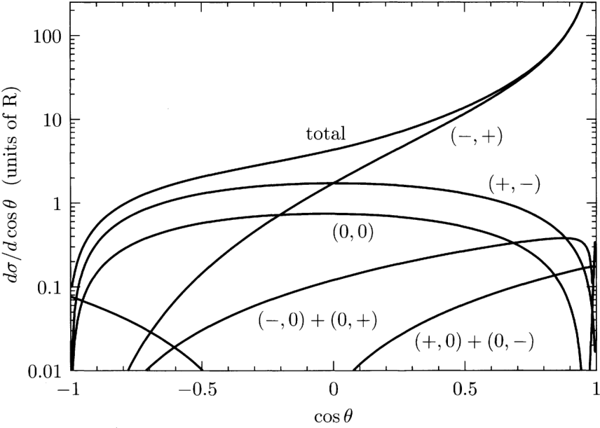
(a) Using explicit polarization vectors, work out the amplitudes for e+e−→W+W− from left- and right-handed electrons to states in which the W+ and W− have definite helicity. For the cases in which both W bosons have longitudinal polarization, verify that Eq. (21.99) gives the correct high-energy limit for right-handed electrons, and verify the complete expression (21.108) for left-handed electrons. For the cases in which one W is longitudinally polarized and the second is transversely polarized, show that the individual diagrams give contributions to the amplitudes that grow like s, but that the complete amplitudes fall as 1/s.
(b) Show that the contributions to eL−eR+→W−W+ found in part (a) reproduce Fig. 21.10, and that the differential cross section for eR−eL+→W−W+ is about 30 times smaller. How many of the qualitative features of the figure can you understand physically?
Features reproduced: t-channel dominance for eL (forward peak, (−,+) state), and gauge cancellation for eR.
21.3
Problem 21.3
peskinChapter 21
习题 21.3
来源: 第21章, PDF第773页
21.3 Cross section for duˉ→W−γ. Compute the amplitudes for duˉ→W−γ for the various possible initial and final helicities. Ignore the quark masses. In this approximation, only the annihilation amplitude from dLuˉR is nonzero. Show that the scattering amplitudes for all final helicity combinations vanish at cosθ=−1/3, where θ is the scattering angle in the center-of-mass system. Compute the differential cross section as a function of cosθ.
习题 21.3 - 解答
习题分析与物理背景
本题要求计算过程 duˉ→W−γ 的散射振幅和微分截面。由于 W 玻色子仅与左手夸克耦合(V−A 相互作用),在忽略夸克质量的近似下,初始态夸克必须具有确定的手征性:d 夸克必须是左手的(dL),uˉ 反夸克必须是右手的(uˉR)。因此,唯一非零的初始螺旋度组合为 dLuˉR。
21.4 Dependence of radiative corrections on the Higgs boson mass.
(a) Consider the contributions to weak-interaction radiative corrections involving the physical Higgs boson h0 of the GWS model. The couplings of the h0 were discussed near the end of Section 20.2. Show that, if we ignore terms proportional to the masses of light fermions, the Higgs boson contributes one-loop corrections to the processes considered in Section 21.3 only through vacuum polarization diagrams. It follows that the contributions to vacuum polarization amplitudes that depend on the Higgs boson mass are gauge invariant.
(b) Draw the vacuum polarization diagrams in Feynman-'t Hooft gauge that involve the Higgs boson, and compute the dependence of the various vacuum polarization amplitudes on the Higgs boson mass mh.
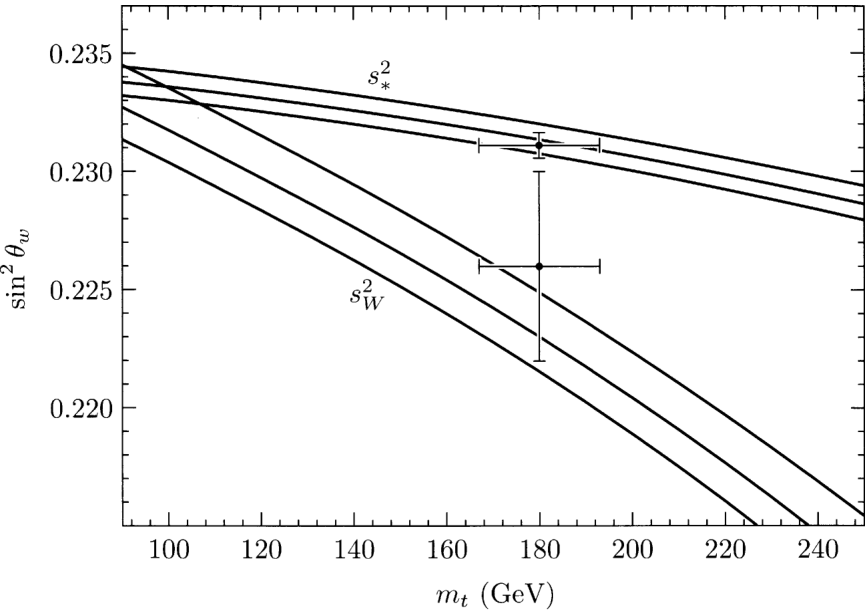
(c) Show that, for mh≫mW, the natural relations discussed in Section 21.3 receive corrections
The effect of varying mh is displayed in Fig. 21.14 and is included as a theoretical uncertainty in the prediction (21.158). More accurate experiments might allow one to predict mh from its effect on electroweak radiative corrections.