习题 7.1 - 解答

---

习题 7.1 分析与解答

对于 $\phi^3$ 理论，其拉格朗日量为： $\mathcal{L} = -\frac{1}{2} \phi (\square + m^2) \phi + \frac{g}{3!} \phi^3$ 由此可以得出动量空间中的费曼规则：

1. 标量传播子：$\frac{i}{p^2 - m^2 + i\epsilon}$
2. 相互作用顶点：$ig$ （相互作用项为 $+\frac{g}{3!}\phi^3$，展开后对称因子 $3!$ 被抵消）

---

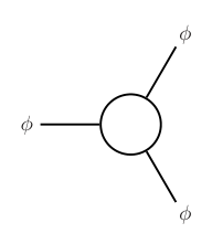
(a) 树图衰变 $\phi \rightarrow \phi \phi$

该过程的树图（Tree-level diagram）由一个单顶点组成，一条动量为 $p_1$ 的入射线分裂为两条动量分别为 $p_2$ 和 $p_3$ 的出射线。 根据费曼规则，该图仅包含一个顶点，没有内部传播子。因此，对应的散射振幅 $i\mathcal{M}$ 直接就是顶点因子： $\boxed{i\mathcal{M}_{\text{tree}} = ig}$

---

(b) 单圈修正振幅

题目给出的单圈图是一个顶点修正图（三角形图）。设入射动量为 $p_1$，出射动量为 $p_2$ 和 $p_3$，满足动量守恒 $p_1 = p_2 + p_3$。 我们在环路中设定动量流向：设连接出射动量 $p_2$ 顶点和入射动量 $p_1$ 顶点的内部线动量为 $k$（从 $p_2$ 顶点流向 $p_1$ 顶点）。 根据动量守恒：

• 从 $p_1$ 顶点流向 $p_3$ 顶点的内部线动量为 $k + p_1$。
• 从 $p_3$ 顶点流向 $p_2$ 顶点的内部线动量为 $(k + p_1) - p_3 = k + p_2$。

该图包含 3 个顶点和 3 条内部传播子，对称因子为 $S=1$。根据费曼规则，写出对应的振幅： $\boxed{i\mathcal{M}_{\text{1-loop}} = (ig)^3 \int \frac{d^4k}{(2\pi)^4} \frac{i}{k^2 - m^2 + i\epsilon} \frac{i}{(k+p_2)^2 - m^2 + i\epsilon} \frac{i}{(k+p_1)^2 - m^2 + i\epsilon}}$

---

(c) 位置空间中的费曼图

在位置空间中，该图对应于格林函数 $G(x_1, x_2, x_3) = \langle 0 | T\{\phi(x_1)\phi(x_2)\phi(x_3)\} | 0 \rangle$ 在微扰展开中的 $\mathcal{O}(g^3)$ 连通项。 由 Dyson 级数展开，我们需要计算： $\frac{i^3}{3!} \int d^4x d^4y d^4z \langle 0 | T\left\{\phi(x_1)\phi(x_2)\phi(x_3) \left(\frac{g}{3!}\phi(x)^3\right) \left(\frac{g}{3!}\phi(y)^3\right) \left(\frac{g}{3!}\phi(z)^3\right)\right\} | 0 \rangle_{\text{conn}}$ 通过 Wick 定理进行收缩以形成三角形图：

1. 将外部点 $x_1, x_2, x_3$ 分别与内部顶点 $x, y, z$ 收缩，共有 $3! = 6$ 种顶点分配方式。假设 $x_1$ 连 $x$，$x_2$ 连 $y$，$x_3$ 连 $z$。
2. 在每个顶点处，有 3 种选择与外部线收缩。
3. 剩下的场形成内部环路：$x$ 连 $y$（$2 \times 2 = 4$ 种），$y$ 连 $z$（$1 \times 2 = 2$ 种），$z$ 连 $x$（$1 \times 1 = 1$ 种）。 总的组合数为 $6 \times (3 \times 3 \times 3) \times (4 \times 2 \times 1) = 1296$。这恰好抵消了分母中的对称因子 $3! \times (3!)^3 = 1296$。

每次收缩产生一个费曼传播子 $D_F(x-y)$。因此，位置空间中该图的表达式为： $\boxed{G(x_1, x_2, x_3) \supset (ig)^3 \int d^4x d^4y d^4z \, D_F(x_1-x) D_F(x_2-y) D_F(x_3-z) D_F(x-y) D_F(y-z) D_F(z-x)}$

---

(d) 使用 LSZ 约化公式推导动量空间振幅

LSZ 约化公式将位置空间的格林函数与 S 矩阵元联系起来： $\langle p_2, p_3 | S | p_1 \rangle = \int d^4x_1 d^4x_2 d^4x_3 \, e^{-ip_1 x_1 + ip_2 x_2 + ip_3 x_3} \left[ i(\square_{x_1} + m^2) \right] \left[ i(\square_{x_2} + m^2) \right] \left[ i(\square_{x_3} + m^2) \right] G(x_1, x_2, x_3)$ 利用传播子的性质 $(\square_w + m^2) D_F(w-v) = -i \delta^{(4)}(w-v)$，即 $i(\square_w + m^2) D_F(w-v) = \delta^{(4)}(w-v)$，作用于外部传播子可得： $\langle p_2, p_3 | S | p_1 \rangle = (ig)^3 \int d^4x d^4y d^4z \, e^{-ip_1 x + ip_2 y + ip_3 z} D_F(x-y) D_F(y-z) D_F(z-x)$ 代入内部传播子的傅里叶变换形式 $D_F(x-y) = \int \frac{d^4k}{(2\pi)^4} \frac{i e^{-ik(x-y)}}{k^2 - m^2 + i\epsilon}$： $\langle p_2, p_3 | S | p_1 \rangle = (ig)^3 \int d^4x d^4y d^4z \int \frac{d^4k_1}{(2\pi)^4} \frac{d^4k_2}{(2\pi)^4} \frac{d^4k_3}{(2\pi)^4} \frac{i e^{-ik_1(y-x)}}{k_1^2 - m^2} \frac{i e^{-ik_2(z-y)}}{k_2^2 - m^2} \frac{i e^{-ik_3(x-z)}}{k_3^2 - m^2} e^{-ip_1 x + ip_2 y + ip_3 z}$ （注：这里定义 $k_1$ 从 $x$ 流向 $y$，$k_2$ 从 $y$ 流向 $z$，$k_3$ 从 $z$ 流向 $x$） 重排指数项并对空间坐标 $x, y, z$ 积分，产生动量守恒的 $\delta$ 函数：

• 对 $x$ 积分：$\int d^4x \, e^{-ix(p_1 - k_1 + k_3)} = (2\pi)^4 \delta^{(4)}(p_1 - k_1 + k_3) \implies k_3 = k_1 - p_1$
• 对 $y$ 积分：$\int d^4y \, e^{iy(p_2 - k_2 + k_1)} = (2\pi)^4 \delta^{(4)}(p_2 - k_2 + k_1) \implies k_2 = k_1 + p_2$
• 对 $z$ 积分：$\int d^4z \, e^{iz(p_3 - k_3 + k_2)} = (2\pi)^4 \delta^{(4)}(p_3 - k_3 + k_2)$

将 $k_2, k_3$ 的关系代入第三个 $\delta$ 函数，得到整体动量守恒： $\delta^{(4)}(p_3 - (k_1 - p_1) + (k_1 + p_2)) = \delta^{(4)}(p_1 - p_2 - p_3)$ 利用两个 $\delta$ 函数积掉 $k_2$ 和 $k_3$，并令 $k_1 = k$，S 矩阵元化为： $\langle p_2, p_3 | S | p_1 \rangle = (2\pi)^4 \delta^{(4)}(p_1 - p_2 - p_3) (ig)^3 \int \frac{d^4k}{(2\pi)^4} \frac{i}{k^2 - m^2} \frac{i}{(k+p_2)^2 - m^2} \frac{i}{(k-p_1)^2 - m^2}$ 由于 $(k-p_1)^2 = (-(k-p_1))^2 = (p_1-k)^2$，若我们作变量代换 $k \rightarrow -k$，则分母变为 $k^2 - m^2$、$(-k+p_2)^2 - m^2 = (k-p_2)^2 - m^2$ 和 $(-k-p_1)^2 - m^2 = (k+p_1)^2 - m^2$。 这与我们在 (b) 中选择的特定动量路由完全等价。根据定义 $\langle f | S | i \rangle = i\mathcal{M} (2\pi)^4 \delta^{(4)}(\sum p)$，提取出振幅： $\boxed{i\mathcal{M} = (ig)^3 \int \frac{d^4k}{(2\pi)^4} \frac{i}{k^2 - m^2 + i\epsilon} \frac{i}{(k+p_2)^2 - m^2 + i\epsilon} \frac{i}{(k+p_1)^2 - m^2 + i\epsilon}}$ 这证明了通过 LSZ 约化位置空间表达式得到的结果与直接使用动量空间费曼规则得到的结果完全一致。

习题 7.2 - 解答

---

习题分析与物理背景

由给定的拉格朗日量 $\mathcal{L} = -\frac{1}{2} \phi \square \phi + \frac{g}{3!} \phi^3 + \frac{1}{6!} \lambda \phi^6$ 可知：

1. 动能项为 $-\frac{1}{2} \phi \square \phi$，没有质量项（即 $m^2=0$），因此该标量场 $\phi$ 描述的是无质量粒子，满足在壳条件 $p^2 = 0$。
2. 相互作用项提供了两种顶点：
   • 3线顶点（3-point vertex），费曼规则为 $ig$。
   • 6线顶点（6-point vertex），费曼规则为 $i\lambda$。

对于 $2 \rightarrow 4$ 散射过程，设初态动量为 $p_1, p_2$，末态动量为 $p_3, p_4, p_5, p_6$。总动量守恒要求 $P_{in} = p_1 + p_2 = \sum_{i=3}^6 p_i = P_{out}$。

---

1. 连通图 (Connected Diagram) 的贡献

连通图由单个 6线顶点构成，2个初态粒子和4个末态粒子直接交汇于一点。 根据费曼规则，6线顶点自带因子 $i\lambda$。由于拉格朗日量中的相互作用项为 $\frac{\lambda}{6!}\phi^6$，6个外线与顶点收缩共有 $6!$ 种组合，恰好抵消分母的 $6!$，因此对称因子为 1。

该连通图的 S 矩阵元为： $S_c = i\lambda (2\pi)^4 \delta^4\left(p_1 + p_2 - \sum_{i=3}^6 p_i\right)$ 提取出不变矩阵元 $\mathcal{M}_c$（定义为 $S_c = i(2\pi)^4\delta^4(P_{in}-P_{out})\mathcal{M}_c$）： $\boxed{\mathcal{M}_c = \lambda}$

---

2. 非连通图 (Disconnected Diagram) 的贡献

非连通图要求过程在拓扑上分离。对于 $2 \rightarrow 4$ 过程且仅使用 3线顶点，最低阶的非连通图只能由两个独立的 $1 \rightarrow 2$ 子过程组成（即每个初态粒子分别衰变为两个末态粒子）。

设末态粒子集合为 $\{3, 4, 5, 6\}$。我们需要将其划分为两个包含2个粒子的子集，分别与 $p_1$ 和 $p_2$ 关联。从4个末态粒子中选2个与 $p_1$ 关联的方式有 $\binom{4}{2} = 6$ 种。这 6 种排列分别为：

1. $p_1 \rightarrow p_3 + p_4$, $p_2 \rightarrow p_5 + p_6$
2. $p_1 \rightarrow p_5 + p_6$, $p_2 \rightarrow p_3 + p_4$
3. $p_1 \rightarrow p_3 + p_5$, $p_2 \rightarrow p_4 + p_6$
4. $p_1 \rightarrow p_4 + p_6$, $p_2 \rightarrow p_3 + p_5$
5. $p_1 \rightarrow p_3 + p_6$, $p_2 \rightarrow p_4 + p_5$
6. $p_1 \rightarrow p_4 + p_5$, $p_2 \rightarrow p_3 + p_6$

对于任意一种划分（例如 $p_1 \rightarrow p_a + p_b$ 且 $p_2 \rightarrow p_c + p_d$），其 S 矩阵元是两个子过程 S 矩阵元的乘积。每个 3线顶点贡献 $ig$。 因此，总的非连通图 S 矩阵元为这 6 种可能性的叠加： $\boxed{ S_{disc} = -g^2 \sum_{\text{6 perms}} (2\pi)^4 \delta^4(p_1 - p_a - p_b) (2\pi)^4 \delta^4(p_2 - p_c - p_d) }$

---

3. 证明两图之间无干涉 (No Interference)

散射截面或跃迁概率正比于 $|S_{fi}|^2 = |S_c + S_{disc}|^2$。干涉项正比于 $S_c S_{disc}^* + c.c.$。 我们来分析干涉项 $S_c S_{disc}^*$ 的结构。取 $S_{disc}$ 中的任意一项（例如 $p_1 \rightarrow p_a + p_b$），干涉项包含如下的狄拉克 $\delta$ 函数乘积： $S_c S_{disc}^* \propto \delta^4(p_1 + p_2 - p_a - p_b - p_c - p_d) \times \delta^4(p_1 - p_a - p_b) \times \delta^4(p_2 - p_c - p_d)$ 由于后两个 $\delta$ 函数同时成立时，第一个全局动量守恒 $\delta$ 函数必然成立，我们可以将全局动量守恒因子提取出来，干涉项在相空间积分中会留下一个额外的约束： $\text{Interference} \propto \int d\Pi_4 \delta^4(p_1 - p_a - p_b)$ 其中 $d\Pi_4$ 是 4 体末态的洛伦兹不变相空间。上述积分等价于要求在相空间中计算一个无质量粒子 $p_1$ 衰变为两个无质量粒子 $p_a, p_b$ 的 2 体相空间体积： $\int \frac{d^3 p_a}{(2\pi)^3 2E_a} \frac{d^3 p_b}{(2\pi)^3 2E_b} \delta^4(p_1 - p_a - p_b)$

运动学分析： 由于场 $\phi$ 无质量，所有外线均满足 $p^2 = 0$。 由 $\delta$ 函数约束 $p_1 = p_a + p_b$，两边平方得： $p_1^2 = (p_a + p_b)^2 \implies 0 = p_a^2 + p_b^2 + 2p_a \cdot p_b \implies 0 = 2p_a \cdot p_b$ 展开点积 $p_a \cdot p_b$： $p_a \cdot p_b = E_a E_b - \vec{p}_a \cdot \vec{p}_b = E_a E_b (1 - \cos\theta) = 0$ 因为 $E_a, E_b > 0$，该等式成立的唯一条件是 $\cos\theta = 1$，即末态粒子 $p_a$ 和 $p_b$ 必须严格共线（Collinear）。

在相空间积分中，严格共线的参数空间维度比全相空间低，其测度为零（Measure zero）。因此，该相空间积分严格等于 0。 （注：从更一般的 S 矩阵理论来看，连通图与非连通图具有不同的动量守恒 $\delta$ 函数结构，它们在物理相空间中的重叠测度始终为零，故在计算可观测的散射截面时互不干涉。）

$\boxed{ \int d\Pi_4 \left( S_c S_{disc}^* + S_c^* S_{disc} \right) = 0 \implies \text{There is no interference between the two diagrams.} }$

习题 7.3 - 解答

---

(a) 树图分析 (Tree-level diagrams)

由拉格朗日量 $\mathcal{L} \supset e m_e A_0 \phi_e \phi_e$ 可知，该理论包含一个由两个标量电子 $\phi_e$ 和一个标量光子 $A_0$ 组成的三线顶点。对于 $e^-(p_1) e^-(p_2) \rightarrow e^-(p_3) e^-(p_4)$ 散射过程，在树图阶（tree-level）可以通过交换 $A_0$ 场画出三个费曼图：

1. $s$-通道 (s-channel)：两个入射电子 $p_1, p_2$ 湮灭产生一个虚 $A_0$ 玻色子，随后该 $A_0$ 衰变为两个出射电子 $p_3, p_4$。
2. $t$-通道 (t-channel)：入射电子 $p_1$ 发射一个虚 $A_0$ 玻色子后变为出射电子 $p_3$，同时入射电子 $p_2$ 吸收该 $A_0$ 后变为出射电子 $p_4$。
3. $u$-通道 (u-channel)：与 $t$-通道类似，但出射电子发生交换，即 $p_1$ 发射 $A_0$ 后变为 $p_4$，$p_2$ 吸收 $A_0$ 后变为 $p_3$。

(b) 真实 QED 中被禁戒的图

在真实的量子电动力学（QED）中，$s$-通道图是被禁戒的。 物理原因：真实的电子带有守恒的 $U(1)$ 电荷。$s$-通道顶点 $e^- e^- \rightarrow \gamma$ 要求两个带负电的电子湮灭成一个电中性的光子，这违背了电荷守恒定律（$-2 \neq 0$）。

(c) 计算 $t$-通道与 $u$-通道振幅

根据拉格朗日量，相互作用项为 $e m_e A_0 \phi_e \phi_e$。由于 $\phi_e$ 是实标量场，包含两个全同场，顶点的费曼规则为 $2 i e m_e$。$A_0$ 场的动能项为 $-\frac{1}{2} A_0 \square A_0$，其传播子为 $\frac{i}{q^2}$。

对于 $t$-通道，动量转移为 $q^2 = t$： $-i \mathcal{M}_t = (2 i e m_e) \frac{i}{t} (2 i e m_e) = \frac{-4 i e^2 m_e^2}{t} \implies \mathcal{M}_t = \frac{4 e^2 m_e^2}{t}$

对于 $u$-通道，动量转移为 $q^2 = u$： $-i \mathcal{M}_u = (2 i e m_e) \frac{i}{u} (2 i e m_e) = \frac{-4 i e^2 m_e^2}{u} \implies \mathcal{M}_u = \frac{4 e^2 m_e^2}{u}$

由于电子实际上是费米子，交换两个全同的末态费米子会引入一个相对负号。因此，总散射振幅为： $\boxed{ \mathcal{M} = \mathcal{M}_t - \mathcal{M}_u = 4 e^2 m_e^2 \left( \frac{1}{t} - \frac{1}{u} \right) }$

(d) 考虑自旋守恒的 16 种构型

在非相对论极限下，软光子无法带走自旋角动量，因此每条费米子线在顶点处的自旋必须守恒。设过程为 $|\sigma_1 \sigma_2\rangle \rightarrow |\sigma_3 \sigma_4\rangle$。

• $t$-通道连接 $1 \rightarrow 3$ 和 $2 \rightarrow 4$，要求 $\sigma_1 = \sigma_3$ 且 $\sigma_2 = \sigma_4$。
• $u$-通道连接 $1 \rightarrow 4$ 和 $2 \rightarrow 3$，要求 $\sigma_1 = \sigma_4$ 且 $\sigma_2 = \sigma_3$。
• $s$-通道在真实物理中被禁戒，不提供贡献。

在 16 种可能的自旋构型中：

1. 同时获得 $t$-通道和 $u$-通道贡献（2种）： $|\uparrow \uparrow\rangle \rightarrow |\uparrow \uparrow\rangle$ $|\downarrow \downarrow\rangle \rightarrow |\downarrow \downarrow\rangle$
2. 仅获得 $t$-通道贡献（2种）： $|\uparrow \downarrow\rangle \rightarrow |\uparrow \downarrow\rangle$ $|\downarrow \uparrow\rangle \rightarrow |\downarrow \uparrow\rangle$
3. 仅获得 $u$-通道贡献（2种）： $|\uparrow \downarrow\rangle \rightarrow |\downarrow \uparrow\rangle$ $|\downarrow \uparrow\rangle \rightarrow |\uparrow \downarrow\rangle$
4. 被禁戒的过程（10种）： 任何不满足上述自旋守恒条件的构型均被禁戒（例如 $|\uparrow \uparrow\rangle \rightarrow |\uparrow \downarrow\rangle$, $|\uparrow \downarrow\rangle \rightarrow |\uparrow \uparrow\rangle$ 等）。

(e) 非极化微分散射截面 $\frac{d\sigma}{d\cos\theta}$

对于非极化束流，我们需要对初态自旋求平均（除以 4），并对末态自旋求和。利用 (d) 中的分析，非零振幅的平方和为： $\sum |\mathcal{M}|^2 = 2 |\mathcal{M}_t - \mathcal{M}_u|^2 + 2 |\mathcal{M}_t|^2 + 2 |-\mathcal{M}_u|^2$ $\overline{|\mathcal{M}|^2} = \frac{1}{4} \sum |\mathcal{M}|^2 = \mathcal{M}_t^2 + \mathcal{M}_u^2 - \mathcal{M}_t \mathcal{M}_u$

代入 $\mathcal{M}_t$ 和 $\mathcal{M}_u$ 的表达式： $\overline{|\mathcal{M}|^2} = 16 e^4 m_e^4 \left( \frac{1}{t^2} + \frac{1}{u^2} - \frac{1}{tu} \right)$

在质心系（CM）中，设三维动量大小为 $p$。运动学变量为： $t = -2p^2(1 - \cos\theta), \quad u = -2p^2(1 + \cos\theta)$ 其中 $p^2 = \frac{E_{\text{CM}}^2}{4} - m_e^2$。代入 $\overline{|\mathcal{M}|^2}$ 中化简括号内的角分布部分： $\frac{1}{t^2} + \frac{1}{u^2} - \frac{1}{tu} = \frac{1}{4p^4} \left[ \frac{1}{(1-\cos\theta)^2} + \frac{1}{(1+\cos\theta)^2} - \frac{1}{1-\cos^2\theta} \right]$ $= \frac{1}{4p^4} \left[ \frac{(1+\cos\theta)^2 + (1-\cos\theta)^2 - (1-\cos^2\theta)}{\sin^4\theta} \right] = \frac{1}{4p^4} \frac{1 + 3\cos^2\theta}{\sin^4\theta}$ 因此，自旋平均后的振幅平方为： $\overline{|\mathcal{M}|^2} = \frac{4 e^4 m_e^4}{p^4} \frac{1 + 3\cos^2\theta}{\sin^4\theta}$

微分散射截面公式为 $\frac{d\sigma}{d\Omega} = \frac{1}{64\pi^2 E_{\text{CM}}^2} \overline{|\mathcal{M}|^2}$。由于 $d\Omega = 2\pi d\cos\theta$，我们有： $\frac{d\sigma}{d\cos\theta} = \frac{2\pi}{64\pi^2 E_{\text{CM}}^2} \overline{|\mathcal{M}|^2} = \frac{1}{32\pi E_{\text{CM}}^2} \frac{4 e^4 m_e^4}{p^4} \frac{1 + 3\cos^2\theta}{\sin^4\theta} = \frac{e^4 m_e^4}{8\pi E_{\text{CM}}^2 p^4} \frac{1 + 3\cos^2\theta}{\sin^4\theta}$

将 $p^4 = \frac{(E_{\text{CM}}^2 - 4m_e^2)^2}{16}$ 代入，得到最终的微分散射截面： $\boxed{ \frac{d\sigma}{d\cos\theta} = \frac{2 e^4 m_e^4}{\pi E_{\text{CM}}^2 (E_{\text{CM}}^2 - 4m_e^2)^2} \frac{1 + 3\cos^2\theta}{\sin^4\theta} }$ (注：若使用精细结构常数 $\alpha = \frac{e^2}{4\pi}$，系数可写为 $\frac{32 \pi \alpha^2 m_e^4}{E_{\text{CM}}^2 (E_{\text{CM}}^2 - 4m_e^2)^2}$)

角分布草图说明 (Sketch of the angular distribution)： 角分布由形状函数 $f(\theta) = \frac{1 + 3\cos^2\theta}{\sin^4\theta}$ 决定。

• 在 $\theta \rightarrow 0$（前向散射）和 $\theta \rightarrow \pi$（后向散射）时，由于分母 $\sin^4\theta \rightarrow 0$，截面发生强烈的库仑发散（趋于正无穷）。
• 函数在 $\theta = \pi/2$ 处取得全局极小值，此时 $f(\pi/2) = 1$。
• 整体分布关于 $\theta = \pi/2$ 呈对称的 U 型曲线。

习题 7.4 - 解答

---

物理背景与题目分析

在标准的量子场论微扰展开中，通常将包含质量项的二次型部分作为自由哈密顿量 $H_0$，从而得到带有质量的传播子。本题要求我们改变微扰展开的基点：将无质量的动能项作为自由哈密顿量 $H_0$，而将质量项视为一种“相互作用” $H_{\text{int}}$。

根据题目给定的哈密顿量： $H_0 = \frac{1}{2} \phi \square \phi, \quad H_{\text{int}} = \frac{1}{2} m^2 \phi^2$ 对应的拉格朗日量密度为 $\mathcal{L}_0 = -\frac{1}{2} \phi \square \phi$（等价于 $\frac{1}{2}(\partial_\mu \phi)^2$），以及相互作用拉格朗日量 $\mathcal{L}_{\text{int}} = -H_{\text{int}} = -\frac{1}{2} m^2 \phi^2$。

由此可以得出两套费曼规则：

1. 无质量自由传播子：在动量空间中为 $\tilde{D}_0(p) = \frac{i}{p^2 + i\epsilon}$。
2. 质量插入顶点（Mass Insertion Vertex）：由于 $\mathcal{L}_{\text{int}} = -\frac{1}{2} m^2 \phi^2$，包含两个相同的场 $\phi$，其顶点因子为 $2! \times \left(-i \frac{1}{2} m^2\right) = -i m^2$。在费曼图中，该顶点表现为传播子线上打一个叉（$\otimes$）。

---

(a) 绘制费曼图 (Feynman Graphs up to order $m^6$)

计算两点格林函数 $\langle 0|T\{\phi(x)\phi(y)\}|0\rangle$。由于质量插入顶点只包含两个场，它不会产生分支，只会像“念珠”一样串在一条线上。动量在顶点处守恒，因此整条线上流淌着相同的动量 $p$。

直到 $\mathcal{O}(m^6)$ 阶的费曼图如下（用文字与符号结构表示）：

• $\mathcal{O}(m^0)$ 阶：一条从 $y$ 到 $x$ 的无质量传播子。 $x \bullet \xleftarrow{p} \bullet y$
• $\mathcal{O}(m^2)$ 阶：包含 1 个质量插入顶点（$\otimes$）。 $x \bullet \xleftarrow{p} \otimes \xleftarrow{p} \bullet y$
• $\mathcal{O}(m^4)$ 阶：包含 2 个质量插入顶点。 $x \bullet \xleftarrow{p} \otimes \xleftarrow{p} \otimes \xleftarrow{p} \bullet y$
• $\mathcal{O}(m^6)$ 阶：包含 3 个质量插入顶点。 $x \bullet \xleftarrow{p} \otimes \xleftarrow{p} \otimes \xleftarrow{p} \otimes \xleftarrow{p} \bullet y$

---

(b) 计算费曼图 (Evaluate the graphs)

为了方便求和，我们在动量空间中计算这些图的表达式。设外部动量为 $p$。

• $\mathcal{O}(m^0)$ 阶： $\tilde{D}^{(0)}(p) = \frac{i}{p^2 + i\epsilon}$
• $\mathcal{O}(m^2)$ 阶：两个传播子夹着一个顶点。 $\tilde{D}^{(1)}(p) = \frac{i}{p^2 + i\epsilon} (-i m^2) \frac{i}{p^2 + i\epsilon} = \frac{i}{p^2 + i\epsilon} \left( \frac{m^2}{p^2 + i\epsilon} \right)$
• $\mathcal{O}(m^4)$ 阶：三个传播子夹着两个顶点。 $\tilde{D}^{(2)}(p) = \frac{i}{p^2 + i\epsilon} (-i m^2) \frac{i}{p^2 + i\epsilon} (-i m^2) \frac{i}{p^2 + i\epsilon} = \frac{i}{p^2 + i\epsilon} \left( \frac{m^2}{p^2 + i\epsilon} \right)^2$
• $\mathcal{O}(m^6)$ 阶：四个传播子夹着三个顶点。 $\tilde{D}^{(3)}(p) = \frac{i}{p^2 + i\epsilon} \left( \frac{m^2}{p^2 + i\epsilon} \right)^3$

在位置空间中，完整的两点函数是上述动量空间表达式的傅里叶逆变换： $\langle 0|T\{\phi(x)\phi(y)\}|0\rangle = \int \frac{d^4p}{(2\pi)^4} e^{-ip \cdot (x-y)} \left[ \tilde{D}^{(0)}(p) + \tilde{D}^{(1)}(p) + \tilde{D}^{(2)}(p) + \tilde{D}^{(3)}(p) + \dots \right]$

---

(c) 对所有阶求和 (Sum the series to all orders)

将所有阶的动量空间表达式相加，我们得到一个无穷级数： $\tilde{D}(p) = \sum_{n=0}^{\infty} \tilde{D}^{(n)}(p) = \sum_{n=0}^{\infty} \frac{i}{p^2 + i\epsilon} \left( \frac{m^2}{p^2 + i\epsilon} \right)^n$

这是一个首项为 $a = \frac{i}{p^2 + i\epsilon}$，公比为 $r = \frac{m^2}{p^2 + i\epsilon}$ 的等比数列（Geometric series）。利用无穷等比数列求和公式 $\sum_{n=0}^\infty a r^n = \frac{a}{1-r}$，我们得到： $\tilde{D}(p) = \frac{\frac{i}{p^2 + i\epsilon}}{1 - \frac{m^2}{p^2 + i\epsilon}} = \frac{i}{p^2 + i\epsilon - m^2}$

整理分母，得到最终的传播子： $\boxed{ \tilde{D}(p) = \frac{i}{p^2 - m^2 + i\epsilon} }$ 这精确地再现了将质量项包含在自由哈密顿量 $H_0 = \frac{1}{2}\phi \square \phi + \frac{1}{2}m^2 \phi^2$ 中时所得到的标准有质量标量场传播子。

---

(d) 经典情形的重复 (Repeat the exercise classically)

在经典场论中，包含外源 $J(x)$ 的完整作用量为： $S = \int d^4x \left[ -\frac{1}{2}\phi \square \phi - \frac{1}{2}m^2 \phi^2 + J \phi \right]$ 对其变分得到完整的经典运动方程（EOM）： $\square \phi + m^2 \phi = J$

1. 求解无质量传播子（格林函数） 如果我们将质量项视为微扰，未微扰的无质量运动方程为 $\square \phi_0 = J$。 在动量空间中，$\square \to -p^2$，因此无质量方程变为： $-p^2 \tilde{\phi}_0(p) = \tilde{J}(p) \implies \tilde{\phi}_0(p) = -\frac{1}{p^2} \tilde{J}(p)$ 这表明无质量格林函数为 $\tilde{G}_0(p) = -\frac{1}{p^2}$。

2. 引入质量微扰并迭代 将完整的运动方程改写为微扰形式： $\square \phi = J - m^2 \phi$ 在动量空间中，这等价于积分方程： $-p^2 \tilde{\phi}(p) = \tilde{J}(p) - m^2 \tilde{\phi}(p) \implies \tilde{\phi}(p) = -\frac{1}{p^2} \tilde{J}(p) + \frac{m^2}{p^2} \tilde{\phi}(p)$ 我们将上式不断迭代展开（即 Born 级数展开）： $\tilde{\phi}(p) = -\frac{1}{p^2} \tilde{J}(p) + \frac{m^2}{p^2} \left( -\frac{1}{p^2} \tilde{J}(p) + \frac{m^2}{p^2} \tilde{\phi}(p) \right)$ $\tilde{\phi}(p) = -\frac{1}{p^2} \tilde{J}(p) - \frac{m^2}{p^4} \tilde{J}(p) - \frac{m^4}{p^6} \tilde{J}(p) - \dots$

3. 对级数求和 提取公因子 $-\frac{1}{p^2} \tilde{J}(p)$，得到： $\tilde{\phi}(p) = -\frac{1}{p^2} \left[ 1 + \frac{m^2}{p^2} + \left(\frac{m^2}{p^2}\right)^2 + \dots \right] \tilde{J}(p)$ 括号内同样是一个公比为 $\frac{m^2}{p^2}$ 的等比数列。对其求和： $\tilde{\phi}(p) = -\frac{1}{p^2} \left( \frac{1}{1 - \frac{m^2}{p^2}} \right) \tilde{J}(p) = \frac{-1}{p^2 - m^2} \tilde{J}(p)$

4. 验证等价性 如果我们一开始就保留质量项，完整的动量空间运动方程为： $(-p^2 + m^2) \tilde{\phi}(p) = \tilde{J}(p) \implies \tilde{\phi}(p) = \frac{-1}{p^2 - m^2} \tilde{J}(p)$ 这与我们通过无质量格林函数微扰迭代并求和得到的结果完全一致。 $\boxed{ \tilde{\phi}(p) = \frac{-1}{p^2 - m^2} \tilde{J}(p) }$

习题 7.5 - 解答

---

物理背景与题意分析

在量子物理中，“分部积分不影响矩阵元”这一命题的核心在于：物理态的边界条件或能量-动量守恒定律会使得分部积分过程中产生的边界项（或全导数项）严格为零。

根据具体的物理语境，这一命题通常有两种表现形式：

1. 量子力学（空间分部积分）：在计算算符的空间积分矩阵元时，将空间导数从波函数的一部分转移到另一部分，边界项因波函数在无穷远处的衰减而消失。
2. 量子场论（时空分部积分）：在作用量或相互作用哈密顿量中进行时空分部积分，等价于相差一个全导数项 $\partial_\mu \Lambda^\mu$。由于四维动量守恒，该全导数项的 S 矩阵元严格为零。

以下分别给出这两种情况的严谨证明。

---

1. 量子力学中的空间分部积分

设 $\hat{O}$ 为一个包含空间导数的算符，不失一般性，将其写为 $\hat{O} = \hat{A} \partial_i \hat{B}$，其中 $\partial_i = \frac{\partial}{\partial x_i}$。我们需要计算其在初态 $|\psi_i\rangle$ 和末态 $|\psi_f\rangle$ 之间的矩阵元： $M = \langle \psi_f | \hat{O} | \psi_i \rangle = \int_V d^3x \, \psi_f^*(\vec{x}) \hat{A}(\vec{x}) \partial_i \left[ \hat{B}(\vec{x}) \psi_i(\vec{x}) \right]$

利用导数的乘积法则（即分部积分的核心），被积函数可以改写为： $\psi_f^* \hat{A} \partial_i (\hat{B} \psi_i) = \partial_i \left( \psi_f^* \hat{A} \hat{B} \psi_i \right) - \partial_i (\psi_f^* \hat{A}) \hat{B} \psi_i$

将其代入积分中，得到两项： $M = \int_V d^3x \, \partial_i \left[ \psi_f^*(\vec{x}) \hat{A}(\vec{x}) \hat{B}(\vec{x}) \psi_i(\vec{x}) \right] - \int_V d^3x \, \partial_i \left[ \psi_f^*(\vec{x}) \hat{A}(\vec{x}) \right] \hat{B}(\vec{x}) \psi_i(\vec{x})$

对于第一项，利用高斯散度定理，可将体积分转化为包围体积 $V$ 的闭合曲面 $\partial V$ 上的面积分： $\int_V d^3x \, \partial_i \left( \psi_f^* \hat{A} \hat{B} \psi_i \right) = \oint_{\partial V} dS_i \, \psi_f^*(\vec{x}) \hat{A}(\vec{x}) \hat{B}(\vec{x}) \psi_i(\vec{x})$

物理近似与边界条件： 在量子力学中，物理态（如束缚态或波包）必须是平方可积（归一化）的，这意味着当 $|\vec{x}| \to \infty$ 时，波函数 $\psi(\vec{x}) \to 0$。只要算符 $\hat{A}, \hat{B}$ 在无穷远处的发散速度不超过波函数的衰减速度，当积分区域 $V$ 扩展到全空间时，该面积分严格趋于零。

因此，边界项消失，矩阵元的值完全由第二项决定： $\boxed{ \int d^3x \, \psi_f^* \hat{A} \partial_i (\hat{B} \psi_i) = - \int d^3x \, \partial_i (\psi_f^* \hat{A}) \hat{B} \psi_i }$ 这表明，通过分部积分将导数算符转移后，矩阵元的数值保持不变（这本质上也是动量算符 $\hat{p}_i = -i\hbar\partial_i$ 具有厄米性的基础）。

---

2. 量子场论中的时空分部积分与全导数

在量子场论中，分部积分通常体现为在拉格朗日量密度中添加或减去一个四维全导数项 $\partial_\mu \Lambda^\mu(x)$。我们需要证明，全导数项在动量本征态 $|p_i\rangle$ 和 $|p_f\rangle$ 之间的时空积分矩阵元（即对 S 矩阵的贡献）为零。

考虑全导数项的矩阵元： $I = \langle p_f | \int d^4x \, \partial_\mu \Lambda^\mu(x) | p_i \rangle = \int d^4x \, \partial_\mu \langle p_f | \Lambda^\mu(x) | p_i \rangle$

利用时空平移算符 $\hat{P}^\mu$，场算符的平移变换为 $\Lambda^\mu(x) = e^{i\hat{P}\cdot x} \Lambda^\mu(0) e^{-i\hat{P}\cdot x}$。作用于动量本征态（满足 $\hat{P}^\mu |p\rangle = p^\mu |p\rangle$）上，可得： $\langle p_f | \Lambda^\mu(x) | p_i \rangle = \langle p_f | e^{i\hat{P}\cdot x} \Lambda^\mu(0) e^{-i\hat{P}\cdot x} | p_i \rangle = e^{i(p_f - p_i)\cdot x} \langle p_f | \Lambda^\mu(0) | p_i \rangle$

对其求四维散度 $\partial_\mu = \frac{\partial}{\partial x^\mu}$： $\partial_\mu \langle p_f | \Lambda^\mu(x) | p_i \rangle = i(p_f - p_i)_\mu e^{i(p_f - p_i)\cdot x} \langle p_f | \Lambda^\mu(0) | p_i \rangle$

将此结果代回时空积分中： $I = \int d^4x \, i(p_f - p_i)_\mu e^{i(p_f - p_i)\cdot x} \langle p_f | \Lambda^\mu(0) | p_i \rangle$

对时空坐标 $x$ 的积分会产生一个狄拉克 $\delta$ 函数，体现了能量-动量守恒： $\int d^4x \, e^{i(p_f - p_i)\cdot x} = (2\pi)^4 \delta^{(4)}(p_f - p_i)$

因此，矩阵元化简为： $I = i(2\pi)^4 \left[ (p_f - p_i)_\mu \delta^{(4)}(p_f - p_i) \right] \langle p_f | \Lambda^\mu(0) | p_i \rangle$

计算技巧与结论： 根据狄拉克 $\delta$ 函数的基本性质 $x \delta(x) \equiv 0$，方括号中的项 $(p_f - p_i)_\mu \delta^{(4)}(p_f - p_i)$ 严格为零。这意味着： $\boxed{ \int d^4x \langle p_f | \partial_\mu \Lambda^\mu(x) | p_i \rangle = 0 }$ 由此得证，在作用量中进行分部积分（即相差一个全导数项）不会对任何物理散射过程的矩阵元产生影响。