13.1

Problem 13.1

schwarzChapter 13

习题 13.1

来源: 第13章, PDF第248页


13.1 Of the tree-level processes in QED, Møller scattering (eeeee^- e^- \rightarrow e^- e^-) is especially interesting because it involves identical particles. (a) Calculate the spin-averaged differential cross section for Møller scattering, eeeee^- e^- \rightarrow e^- e^-. Express your answer in terms of s,t,us, t, u and mem_e. (b) Show that in the non-relativistic limit you get what we guessed by spin-conservation arguments in Problem 7.3:

dσdΩ=me4α2ECM2p4(1+3cos2θsin4θ),p2=(ECM2)2me2.(13.162)\frac{d\sigma}{d\Omega} = \frac{m_e^4 \alpha^2}{E_{CM}^2 p^4} \left( \frac{1 + 3 \cos^2 \theta}{\sin^4 \theta} \right), \quad p^2 = \left( \frac{E_{CM}}{2} \right)^2 - m_e^2. \tag{13.162}

(c) Simplify the Møller scattering formula in the ultra-relativistic limit (me0m_e \rightarrow 0). [Hint: you should get something proportional to (3+cos2θ)2(3 + \cos^2 \theta)^2.]

习题 13.1 - 解答


(a) 计算 Møller 散射的自旋平均微分散射截面

Møller 散射 (eeeee^- e^- \rightarrow e^- e^-) 包含两个树图级别的费曼图:tt-通道和 uu-通道。设初态动量为 p1,p2p_1, p_2,末态动量为 p3,p4p_3, p_4。由于末态是全同费米子,根据费米-狄拉克统计,交换两个末态粒子会引入一个相对负号。不变振幅 M\mathcal{M} 为:

iM=iMt+iMu=(ie)2[uˉ(p3)γμu(p1)uˉ(p4)γμu(p2)tuˉ(p4)γμu(p1)uˉ(p3)γμu(p2)u]i\mathcal{M} = i\mathcal{M}_t + i\mathcal{M}_u = (-ie)^2 \left[ \frac{\bar{u}(p_3)\gamma^\mu u(p_1) \bar{u}(p_4)\gamma_\mu u(p_2)}{t} - \frac{\bar{u}(p_4)\gamma^\mu u(p_1) \bar{u}(p_3)\gamma_\mu u(p_2)}{u} \right]

其中 Mandelstam 变量定义为 s=(p1+p2)2s = (p_1+p_2)^2t=(p1p3)2t = (p_1-p_3)^2u=(p1p4)2u = (p_1-p_4)^2,且满足 s+t+u=4me2s+t+u = 4m_e^2

对初态自旋求平均并对末态自旋求和,得到自旋平均的振幅平方:

M2=14spinsM2=e44(Tttt2+Tuuu22Ttutu)\overline{|\mathcal{M}|^2} = \frac{1}{4} \sum_{\text{spins}} |\mathcal{M}|^2 = \frac{e^4}{4} \left( \frac{T_{tt}}{t^2} + \frac{T_{uu}}{u^2} - \frac{2T_{tu}}{tu} \right)

利用迹定理计算各项。对于 tt-通道项 TttT_{tt}

Ttt=Tr[(̸p3+me)γμ(̸p1+me)γν]Tr[(̸p4+me)γμ(̸p2+me)γν]=32[(p1p2)(p3p4)+(p1p4)(p2p3)me2(p1p3+p2p4)+2me4]\begin{aligned} T_{tt} &= \text{Tr}[(\not{p}_3+m_e)\gamma^\mu(\not{p}_1+m_e)\gamma^\nu] \text{Tr}[(\not{p}_4+m_e)\gamma_\mu(\not{p}_2+m_e)\gamma_\nu] \\ &= 32 \left[ (p_1 \cdot p_2)(p_3 \cdot p_4) + (p_1 \cdot p_4)(p_2 \cdot p_3) - m_e^2(p_1 \cdot p_3 + p_2 \cdot p_4) + 2m_e^4 \right] \end{aligned}

代入运动学关系 p1p2=p3p4=s2me22p_1 \cdot p_2 = p_3 \cdot p_4 = \frac{s-2m_e^2}{2}p1p4=p2p3=2me2u2p_1 \cdot p_4 = p_2 \cdot p_3 = \frac{2m_e^2-u}{2}p1p3=p2p4=2me2t2p_1 \cdot p_3 = p_2 \cdot p_4 = \frac{2m_e^2-t}{2},化简得:

Ttt=8[(s2me2)2+(u2me2)2+4me2t]T_{tt} = 8 \left[ (s-2m_e^2)^2 + (u-2m_e^2)^2 + 4m_e^2 t \right]

tut \leftrightarrow u 的对称性,可直接写出 uu-通道项:

Tuu=8[(s2me2)2+(t2me2)2+4me2u]T_{uu} = 8 \left[ (s-2m_e^2)^2 + (t-2m_e^2)^2 + 4m_e^2 u \right]

对于干涉项 TtuT_{tu},利用 γ\gamma 矩阵的缩并恒等式(如 γμγνγμ=2γν\gamma^\mu \not{a} \gamma^\nu \not{b} \gamma_\mu = -2\not{b}\gamma^\nu\not{a} 等)计算大迹:

Ttu=Tr[(̸p3+me)γμ(̸p1+me)γν(̸p4+me)γμ(̸p2+me)γν]=32(p1p2)(p3p4)+16me2(p1p2+p1p3+p1p4+p2p3+p2p4+p3p4)32me4=8(s2me2)2+32me2(2s2me2)32me4=8(s28me2s+12me4)=8(s2me2)(s6me2)\begin{aligned} T_{tu} &= \text{Tr}[(\not{p}_3+m_e)\gamma^\mu(\not{p}_1+m_e)\gamma^\nu(\not{p}_4+m_e)\gamma_\mu(\not{p}_2+m_e)\gamma_\nu] \\ &= -32(p_1 \cdot p_2)(p_3 \cdot p_4) + 16m_e^2(p_1 \cdot p_2 + p_1 \cdot p_3 + p_1 \cdot p_4 + p_2 \cdot p_3 + p_2 \cdot p_4 + p_3 \cdot p_4) - 32m_e^4 \\ &= -8(s-2m_e^2)^2 + 32m_e^2(2s-2m_e^2) - 32m_e^4 \\ &= -8(s^2 - 8m_e^2 s + 12m_e^4) = -8(s-2m_e^2)(s-6m_e^2) \end{aligned}

将上述结果代入 M2\overline{|\mathcal{M}|^2},并提取公因子 2e42e^4

M2=2e4[(s2me2)2+(u2me2)2+4me2tt2+(s2me2)2+(t2me2)2+4me2uu2+2(s2me2)(s6me2)tu]\overline{|\mathcal{M}|^2} = 2e^4 \left[ \frac{(s-2m_e^2)^2 + (u-2m_e^2)^2 + 4m_e^2 t}{t^2} + \frac{(s-2m_e^2)^2 + (t-2m_e^2)^2 + 4m_e^2 u}{u^2} + \frac{2(s-2m_e^2)(s-6m_e^2)}{tu} \right]

在质心系中,弹性散射的微分散射截面公式为 dσdΩ=M264π2s\frac{d\sigma}{d\Omega} = \frac{\overline{|\mathcal{M}|^2}}{64\pi^2 s}。代入精细结构常数 α=e24π\alpha = \frac{e^2}{4\pi}(即 e4=16π2α2e^4 = 16\pi^2 \alpha^2),得到:

dσdΩ=α22s[(s2me2)2+(u2me2)2+4me2tt2+(s2me2)2+(t2me2)2+4me2uu2+2(s2me2)(s6me2)tu]\boxed{ \frac{d\sigma}{d\Omega} = \frac{\alpha^2}{2s} \left[ \frac{(s-2m_e^2)^2 + (u-2m_e^2)^2 + 4m_e^2 t}{t^2} + \frac{(s-2m_e^2)^2 + (t-2m_e^2)^2 + 4m_e^2 u}{u^2} + \frac{2(s-2m_e^2)(s-6m_e^2)}{tu} \right] }

(b) 证明非相对论极限下的形式

在非相对论 (NR) 极限下,质心系三维动量 pmep \ll m_e。此时有:

s=ECM2=4(me2+p2)4me2+4p2s = E_{CM}^2 = 4(m_e^2 + p^2) \approx 4m_e^2 + 4p^2
t=2p2(1cosθ),u=2p2(1+cosθ)t = -2p^2(1-\cos\theta), \quad u = -2p^2(1+\cos\theta)

保留到最低阶 O(p0)\mathcal{O}(p^0),计算 (a) 中方括号内各项的分子:

  1. t2t^2 项分子:(s2me2)2+(u2me2)2+4me2t(2me2)2+(2me2)2+0=8me4(s-2m_e^2)^2 + (u-2m_e^2)^2 + 4m_e^2 t \approx (2m_e^2)^2 + (-2m_e^2)^2 + 0 = 8m_e^4
  2. u2u^2 项分子:(s2me2)2+(t2me2)2+4me2u(2me2)2+(2me2)2+0=8me4(s-2m_e^2)^2 + (t-2m_e^2)^2 + 4m_e^2 u \approx (2m_e^2)^2 + (-2m_e^2)^2 + 0 = 8m_e^4
  3. tutu 项分子:2(s2me2)(s6me2)2(2me2)(2me2)=8me42(s-2m_e^2)(s-6m_e^2) \approx 2(2m_e^2)(-2m_e^2) = -8m_e^4

将这些分子与精确的分母代入 M2\overline{|\mathcal{M}|^2} 中:

M22e4[8me44p4(1cosθ)2+8me44p4(1+cosθ)28me44p4(1cos2θ)]=4e4me4p4[1(1cosθ)2+1(1+cosθ)21sin2θ]\begin{aligned} \overline{|\mathcal{M}|^2} &\approx 2e^4 \left[ \frac{8m_e^4}{4p^4(1-\cos\theta)^2} + \frac{8m_e^4}{4p^4(1+\cos\theta)^2} - \frac{8m_e^4}{4p^4(1-\cos^2\theta)} \right] \\ &= \frac{4e^4 m_e^4}{p^4} \left[ \frac{1}{(1-\cos\theta)^2} + \frac{1}{(1+\cos\theta)^2} - \frac{1}{\sin^2\theta} \right] \end{aligned}

化简括号内的三角函数部分:

(1+cosθ)2+(1cosθ)2sin4θsin2θsin4θ=2+2cos2θ(1cos2θ)sin4θ=1+3cos2θsin4θ\frac{(1+\cos\theta)^2 + (1-\cos\theta)^2}{\sin^4\theta} - \frac{\sin^2\theta}{\sin^4\theta} = \frac{2 + 2\cos^2\theta - (1-\cos^2\theta)}{\sin^4\theta} = \frac{1 + 3\cos^2\theta}{\sin^4\theta}

因此,微分散射截面为:

dσdΩ=164π2ECM2(4(16π2α2)me4p41+3cos2θsin4θ)\frac{d\sigma}{d\Omega} = \frac{1}{64\pi^2 E_{CM}^2} \left( \frac{4(16\pi^2 \alpha^2) m_e^4}{p^4} \frac{1 + 3\cos^2\theta}{\sin^4\theta} \right)

化简即得:

dσdΩ=me4α2ECM2p4(1+3cos2θsin4θ)\boxed{ \frac{d\sigma}{d\Omega} = \frac{m_e^4 \alpha^2}{E_{CM}^2 p^4} \left( \frac{1 + 3 \cos^2 \theta}{\sin^4 \theta} \right) }

(c) 极端相对论极限下的化简

在极端相对论 (UR) 极限下,me0m_e \rightarrow 0。此时 Mandelstam 变量满足 s+t+u=0s+t+u = 0,且:

t=s2(1cosθ),u=s2(1+cosθ)t = -\frac{s}{2}(1-\cos\theta), \quad u = -\frac{s}{2}(1+\cos\theta)

me=0m_e = 0 代入 (a) 的结果中:

dσdΩ=α22s(s2+u2t2+s2+t2u2+2s2tu)\frac{d\sigma}{d\Omega} = \frac{\alpha^2}{2s} \left( \frac{s^2+u^2}{t^2} + \frac{s^2+t^2}{u^2} + \frac{2s^2}{tu} \right)

提取公分母 t2u2t^2 u^2 并利用 s=(t+u)s = -(t+u) 进行代数变形:

s2+u2t2+s2+t2u2+2s2tu=s2(1t+1u)2+u4+t4t2u2=s2(t+utu)2+u4+t4t2u2=s4+t4+u4t2u2\begin{aligned} \frac{s^2+u^2}{t^2} + \frac{s^2+t^2}{u^2} + \frac{2s^2}{tu} &= s^2 \left( \frac{1}{t} + \frac{1}{u} \right)^2 + \frac{u^4 + t^4}{t^2 u^2} \\ &= s^2 \left( \frac{t+u}{tu} \right)^2 + \frac{u^4 + t^4}{t^2 u^2} = \frac{s^4 + t^4 + u^4}{t^2 u^2} \end{aligned}

ttuuθ\theta 表达,计算分子和分母: 分母:t2u2=(s24sin2θ)2=s416sin4θt^2 u^2 = \left( \frac{s^2}{4} \sin^2\theta \right)^2 = \frac{s^4}{16} \sin^4\theta 分子:

s4+t4+u4=s4+s416(1cosθ)4+s416(1+cosθ)4=s4+s48(1+6cos2θ+cos4θ)=s48(9+6cos2θ+cos4θ)=s48(3+cos2θ)2\begin{aligned} s^4 + t^4 + u^4 &= s^4 + \frac{s^4}{16}(1-\cos\theta)^4 + \frac{s^4}{16}(1+\cos\theta)^4 \\ &= s^4 + \frac{s^4}{8}(1 + 6\cos^2\theta + \cos^4\theta) \\ &= \frac{s^4}{8}(9 + 6\cos^2\theta + \cos^4\theta) = \frac{s^4}{8}(3 + \cos^2\theta)^2 \end{aligned}

将分子分母代回截面公式:

dσdΩ=α22ss48(3+cos2θ)2s416sin4θ=α22s2(3+cos2θ)2sin4θ\frac{d\sigma}{d\Omega} = \frac{\alpha^2}{2s} \frac{\frac{s^4}{8}(3 + \cos^2\theta)^2}{\frac{s^4}{16} \sin^4\theta} = \frac{\alpha^2}{2s} \frac{2(3 + \cos^2\theta)^2}{\sin^4\theta}

最终得到极端相对论极限下的简洁形式:

dσdΩ=α2s(3+cos2θ)2sin4θ\boxed{ \frac{d\sigma}{d\Omega} = \frac{\alpha^2}{s} \frac{(3 + \cos^2 \theta)^2}{\sin^4 \theta} }
13.2

Problem 13.2

schwarzChapter 13

习题 13.2

来源: 第13章, PDF第248页


13.2 Derive Eq. (13.103). It may be helpful to use the formula for scattering in the target rest frame derived in Problem 5.1.


Referenced Equations:

Equation (13.103):

dσdΩ=e464π2E2sin4θ2EE(cos2θ2+EEmpsin2θ2),meE,(13.103)\frac{d\sigma}{d\Omega} = \frac{e^4}{64\pi^2 E^2 \sin^4 \frac{\theta}{2}} \frac{E'}{E} \left( \cos^2 \frac{\theta}{2} + \frac{E - E'}{m_p} \sin^2 \frac{\theta}{2} \right), \quad m_e \ll E, \tag{13.103}

Equation (5.1):

Sfi=fSi(5.1)S_{fi} = \langle f | S | i \rangle \tag{5.1}

习题 13.2 - 解答


为了推导无结构质子(即将其视为点状 Dirac 粒子)与电子的弹性散射截面公式 (13.103),我们需要从运动学、相空间积分以及矩阵元平方的迹计算三个方面进行严谨的推导。

1. 运动学分析

设在靶静止系(实验室系)中,初始电子、初始质子、末态电子和末态质子的四维动量分别为: p1=(E,p1),p2=(mp,0),p3=(E,p3),p4=(E4,p4)p_1 = (E, \vec{p}_1), \quad p_2 = (m_p, \vec{0}), \quad p_3 = (E', \vec{p}_3), \quad p_4 = (E_4, \vec{p}_4) 由于 meEm_e \ll E,我们近似认为电子是无质量的,即 p12=p320p_1^2 = p_3^2 \approx 0。 动量转移的平方 q2q^2 可以通过电子的动量表示为: q2=(p1p3)2=2p1p3=2EE(1cosθ)=4EEsin2θ2q^2 = (p_1 - p_3)^2 = -2p_1 \cdot p_3 = -2EE'(1 - \cos\theta) = -4EE' \sin^2 \frac{\theta}{2} 同时,q2q^2 也可以通过质子的动量表示。利用能量守恒 E4=E+mpEE_4 = E + m_p - E',有: q2=(p4p2)2=2mp22p2p4=2mp22mpE4=2mp(EE)q^2 = (p_4 - p_2)^2 = 2m_p^2 - 2p_2 \cdot p_4 = 2m_p^2 - 2m_p E_4 = -2m_p(E - E') 联立上述两个 q2q^2 的表达式,我们可以得到能量转移与散射角的关系: p1p3=mp(EE)    EE=2EEmpsin2θ2p_1 \cdot p_3 = m_p(E - E') \quad \implies \quad E - E' = \frac{2EE'}{m_p} \sin^2 \frac{\theta}{2}

2. 靶静止系下的相空间与截面公式

根据 Problem 5.1 的结论,对于 222 \to 2 散射,靶静止系下的微分截面公式可以由费米黄金定则出发推导。通用的微分散射截面为: dσ=14Empd3p3(2π)32Ed3p4(2π)32E4(2π)4δ4(p1+p2p3p4)M2d\sigma = \frac{1}{4 E m_p} \int \frac{d^3 p_3}{(2\pi)^3 2 E'} \frac{d^3 p_4}{(2\pi)^3 2 E_4} (2\pi)^4 \delta^4(p_1 + p_2 - p_3 - p_4) \overline{|\mathcal{M}|^2}p4\vec{p}_4 积分消除三维 δ\delta 函数后,得到: dσdΩ=164π2EmpE2dEEE4δ(E+mpEE4)M2\frac{d\sigma}{d\Omega} = \frac{1}{64\pi^2 E m_p} \int \frac{E'^2 dE'}{E' E_4} \delta(E + m_p - E' - E_4) \overline{|\mathcal{M}|^2} 其中 E4=mp2+E2+E22EEcosθE_4 = \sqrt{m_p^2 + E^2 + E'^2 - 2EE'\cos\theta}。定义 δ\delta 函数中的自变量为 f(E)=E+mpEE4f(E') = E + m_p - E' - E_4,对其求导: fE=1+EEcosθE4=E4+EEcosθE4=mp+E(1cosθ)E4\left| \frac{\partial f}{\partial E'} \right| = 1 + \frac{E' - E \cos\theta}{E_4} = \frac{E_4 + E' - E \cos\theta}{E_4} = \frac{m_p + E(1 - \cos\theta)}{E_4} 利用运动学关系 E(1cosθ)=mp(EE)EE(1 - \cos\theta) = \frac{m_p(E - E')}{E'},上式可化简为: fE=mp+mp(EE)EE4=mpEEE4\left| \frac{\partial f}{\partial E'} \right| = \frac{m_p + \frac{m_p(E - E')}{E'}}{E_4} = \frac{m_p E}{E' E_4} 完成对 EE' 的积分,引入雅可比因子 fE1=EE4mpE\left| \frac{\partial f}{\partial E'} \right|^{-1} = \frac{E' E_4}{m_p E},得到靶静止系下的截面公式: dσdΩ=164π2EmpEE4EE4mpEM2=164π2mp2(EE)2M2\frac{d\sigma}{d\Omega} = \frac{1}{64\pi^2 E m_p} \frac{E'}{E_4} \frac{E' E_4}{m_p E} \overline{|\mathcal{M}|^2} = \frac{1}{64\pi^2 m_p^2} \left( \frac{E'}{E} \right)^2 \overline{|\mathcal{M}|^2}

3. 矩阵元平方计算

将质子视为点状 Dirac 粒子,自旋平均的矩阵元平方为: M2=e4q4Lμν(e)L(p)μν\overline{|\mathcal{M}|^2} = \frac{e^4}{q^4} L_{\mu\nu}^{(e)} L^{\mu\nu}_{(p)} 其中电子和质子的轻子张量(迹)分别为: Lμν(e)=12Tr[γμ̸p1γν̸p3]=2(p1μp3ν+p1νp3μgμνp1p3)L_{\mu\nu}^{(e)} = \frac{1}{2} \text{Tr}[\gamma_\mu \not{p}_1 \gamma_\nu \not{p}_3] = 2 (p_{1\mu} p_{3\nu} + p_{1\nu} p_{3\mu} - g_{\mu\nu} p_1 \cdot p_3) L(p)μν=12Tr[γμ(̸p2+mp)γν(̸p4+mp)]=2(p2μp4ν+p2νp4μgμν(p2p4mp2))L^{\mu\nu}_{(p)} = \frac{1}{2} \text{Tr}[\gamma^\mu (\not{p}_2 + m_p) \gamma^\nu (\not{p}_4 + m_p)] = 2 (p_2^\mu p_4^\nu + p_2^\nu p_4^\mu - g^{\mu\nu} (p_2 \cdot p_4 - m_p^2)) 将两者收缩,利用 gμνgμν=4g_{\mu\nu}g^{\mu\nu}=4,可得: Lμν(e)L(p)μν=8[(p1p2)(p3p4)+(p1p4)(p3p2)mp2(p1p3)]L_{\mu\nu}^{(e)} L^{\mu\nu}_{(p)} = 8 \big[ (p_1 \cdot p_2)(p_3 \cdot p_4) + (p_1 \cdot p_4)(p_3 \cdot p_2) - m_p^2 (p_1 \cdot p_3) \big] 接下来计算各个四维内积。已知 p1p2=Empp_1 \cdot p_2 = E m_pp3p2=Empp_3 \cdot p_2 = E' m_p,且 p1p3=mp(EE)p_1 \cdot p_3 = m_p(E - E')。利用四动量守恒 p4=p1+p2p3p_4 = p_1 + p_2 - p_3,有: p3p4=p3(p1+p2p3)=p1p3+p2p3=mp(EE)+mpE=mpEp_3 \cdot p_4 = p_3 \cdot (p_1 + p_2 - p_3) = p_1 \cdot p_3 + p_2 \cdot p_3 = m_p(E - E') + m_p E' = m_p E p1p4=p1(p1+p2p3)=p1p2p1p3=mpEmp(EE)=mpEp_1 \cdot p_4 = p_1 \cdot (p_1 + p_2 - p_3) = p_1 \cdot p_2 - p_1 \cdot p_3 = m_p E - m_p(E - E') = m_p E' 代入张量收缩的结果中: Lμν(e)L(p)μν=8[(Emp)(mpE)+(mpE)(Emp)mp2(2EEsin2θ2)]=8mp2(E2+E22EEsin2θ2)L_{\mu\nu}^{(e)} L^{\mu\nu}_{(p)} = 8 \big[ (E m_p)(m_p E) + (m_p E')(E' m_p) - m_p^2 \left( 2EE' \sin^2 \frac{\theta}{2} \right) \big] = 8 m_p^2 \left( E^2 + E'^2 - 2EE' \sin^2 \frac{\theta}{2} \right) 为了凑出目标公式的形式,我们将括号内的项进行代数变形: E2+E22EEsin2θ2=(EE)2+2EEcos2θ2E^2 + E'^2 - 2EE' \sin^2 \frac{\theta}{2} = (E - E')^2 + 2EE' \cos^2 \frac{\theta}{2} 利用运动学关系 (EE)=2EEmpsin2θ2(E - E') = \frac{2EE'}{m_p} \sin^2 \frac{\theta}{2},将 (EE)2(E - E')^2 中的一个 (EE)(E - E') 替换掉: (EE)2+2EEcos2θ2=2EEEEmpsin2θ2+2EEcos2θ2=2EE(cos2θ2+EEmpsin2θ2)(E - E')^2 + 2EE' \cos^2 \frac{\theta}{2} = 2EE' \frac{E - E'}{m_p} \sin^2 \frac{\theta}{2} + 2EE' \cos^2 \frac{\theta}{2} = 2EE' \left( \cos^2 \frac{\theta}{2} + \frac{E - E'}{m_p} \sin^2 \frac{\theta}{2} \right) 因此,张量收缩的最终结果为: Lμν(e)L(p)μν=16mp2EE(cos2θ2+EEmpsin2θ2)L_{\mu\nu}^{(e)} L^{\mu\nu}_{(p)} = 16 m_p^2 E E' \left( \cos^2 \frac{\theta}{2} + \frac{E - E'}{m_p} \sin^2 \frac{\theta}{2} \right)

4. 最终结果组装

q4=16E2E2sin4θ2q^4 = 16 E^2 E'^2 \sin^4 \frac{\theta}{2} 和张量收缩结果代入矩阵元平方中: M2=e416E2E2sin4θ2×16mp2EE(cos2θ2+EEmpsin2θ2)=e4mp2EEsin4θ2(cos2θ2+EEmpsin2θ2)\overline{|\mathcal{M}|^2} = \frac{e^4}{16 E^2 E'^2 \sin^4 \frac{\theta}{2}} \times 16 m_p^2 E E' \left( \cos^2 \frac{\theta}{2} + \frac{E - E'}{m_p} \sin^2 \frac{\theta}{2} \right) = \frac{e^4 m_p^2}{E E' \sin^4 \frac{\theta}{2}} \left( \cos^2 \frac{\theta}{2} + \frac{E - E'}{m_p} \sin^2 \frac{\theta}{2} \right) 最后,将其代入第 2 步推导的截面公式中: dσdΩ=164π2mp2E2E2e4mp2EEsin4θ2(cos2θ2+EEmpsin2θ2)\frac{d\sigma}{d\Omega} = \frac{1}{64\pi^2 m_p^2} \frac{E'^2}{E^2} \frac{e^4 m_p^2}{E E' \sin^4 \frac{\theta}{2}} \left( \cos^2 \frac{\theta}{2} + \frac{E - E'}{m_p} \sin^2 \frac{\theta}{2} \right) 化简后即得到目标方程 (13.103):

dσdΩ=e464π2E2sin4θ2EE(cos2θ2+EEmpsin2θ2)\boxed{ \frac{d\sigma}{d\Omega} = \frac{e^4}{64\pi^2 E^2 \sin^4 \frac{\theta}{2}} \frac{E'}{E} \left( \cos^2 \frac{\theta}{2} + \frac{E - E'}{m_p} \sin^2 \frac{\theta}{2} \right) }
13.3

Problem 13.3

schwarzChapter 13

习题 13.3

来源: 第13章, PDF第248页


13.3 Particle decays. Recall that the decay rate is given by the general formula

dΓ=12E1M2d3p2(2π)32E2d3pn(2π)32En(2π)4δ4(p1p2pn).(13.163)d\Gamma = \frac{1}{2E_1} |\mathcal{M}|^2 \frac{d^3 p_2}{(2\pi)^3 2E_2} \cdots \frac{d^3 p_n}{(2\pi)^3 2E_n} (2\pi)^4 \delta^4(p_1 - p_2 - \cdots - p_n). \tag{13.163}

(a) Evaluate the phase-space integrals for 121 \rightarrow 2 decays. Show that the total rate is

Γ(ϕe+e)=14x216πmϕM2,x=memϕ.(13.164)\Gamma(\phi \rightarrow e^+ e^-) = \frac{\sqrt{1 - 4x^2}}{16\pi m_\phi} |\mathcal{M}|^2, \quad x = \frac{m_e}{m_\phi}. \tag{13.164}

(b) Evaluate Γ\Gamma for a particle ϕ\phi of mass mϕm_\phi decaying to e+ee^+ e^- of mass mem_e if

  1. ϕ\phi is a scalar, with interaction gSϕψˉψg_S \phi \bar{\psi} \psi;
  2. ϕ\phi is a pseudoscalar, with interaction igPϕψˉγ5ψig_P \phi \bar{\psi} \gamma_5 \psi;
  3. ϕ\phi is a vector, with interaction gVϕμψˉγμψg_V \phi_\mu \bar{\psi} \gamma^\mu \psi;
  4. ϕ\phi is an axial vector, with interaction igAϕμψˉγμγ5ψig_A \phi_\mu \bar{\psi} \gamma^\mu \gamma_5 \psi. (c) Breaking news! A collider experiment reports evidence of a new particle that decays only to leptons (τ,μ\tau, \mu and ee) whose mass is around 4 GeV. About 25% of the time it decays to τ+τ\tau^+ \tau^-. What spin and parity might this particle have?

习题 13.3 - 解答


(a) 相空间积分与总衰变率

在衰变粒子 ϕ\phi 的静止参考系中,其四维动量为 p1=(mϕ,0)p_1 = (m_\phi, \vec{0})。设末态正负电子的动量分别为 p2p_2p3p_3。两体相空间积分公式为:

dΠ2=d3p2(2π)32E2d3p3(2π)32E3(2π)4δ4(p1p2p3)\int d\Pi_2 = \int \frac{d^3 p_2}{(2\pi)^3 2E_2} \frac{d^3 p_3}{(2\pi)^3 2E_3} (2\pi)^4 \delta^4(p_1 - p_2 - p_3)

首先对 d3p3d^3 p_3 积分,利用空间动量守恒 δ3(p1p2p3)\delta^3(\vec{p}_1 - \vec{p}_2 - \vec{p}_3),得到 p3=p2\vec{p}_3 = -\vec{p}_2。由于正负电子质量相同(mem_e),它们的能量也相等:E2=E3=p22+me2EE_2 = E_3 = \sqrt{|\vec{p}_2|^2 + m_e^2} \equiv E。相空间积分化简为:

dΠ2=1(2π)2d3p24E2δ(mϕ2E)\int d\Pi_2 = \frac{1}{(2\pi)^2} \int \frac{d^3 p_2}{4E^2} \delta(m_\phi - 2E)

在球坐标系下,d3p2=p22dp2dΩd^3 p_2 = |\vec{p}_2|^2 d|\vec{p}_2| d\Omega。利用关系式 p2dp2=EdE|\vec{p}_2| d|\vec{p}_2| = E dE,并对立体角 dΩd\Omega 积分得到 4π4\pi

dΠ2=4π(2π)2p2EdE4E2δ(mϕ2E)=14πp2EdE12δ(Emϕ2)\int d\Pi_2 = \frac{4\pi}{(2\pi)^2} \int \frac{|\vec{p}_2| E dE}{4E^2} \delta(m_\phi - 2E) = \frac{1}{4\pi} \int \frac{|\vec{p}_2|}{E} dE \frac{1}{2} \delta\left(E - \frac{m_\phi}{2}\right)

积分给出 E=mϕ/2E = m_\phi/2,此时动量大小为 p2=E2me2=mϕ214me2/mϕ2|\vec{p}_2| = \sqrt{E^2 - m_e^2} = \frac{m_\phi}{2}\sqrt{1 - 4m_e^2/m_\phi^2}。定义质量比 x=me/mϕx = m_e/m_\phi,则 p2=mϕ214x2|\vec{p}_2| = \frac{m_\phi}{2}\sqrt{1 - 4x^2}。代入上式得:

dΠ2=18πmϕ214x2mϕ/2=18π14x2\int d\Pi_2 = \frac{1}{8\pi} \frac{\frac{m_\phi}{2}\sqrt{1 - 4x^2}}{m_\phi/2} = \frac{1}{8\pi} \sqrt{1 - 4x^2}

将相空间积分结果代入总衰变率公式 Γ=12mϕM2dΠ2\Gamma = \frac{1}{2m_\phi} |\mathcal{M}|^2 \int d\Pi_2,即可得到:

Γ(ϕe+e)=14x216πmϕM2\boxed{\Gamma(\phi \rightarrow e^+ e^-) = \frac{\sqrt{1 - 4x^2}}{16\pi m_\phi} |\mathcal{M}|^2}

(b) 不同自旋与宇称下的衰变率

在计算中,我们需要对末态自旋求和,并对初态极化(若有)求平均。由运动学关系 p1=p2+p3p_1 = p_2 + p_3,平方后得到 mϕ2=2me2+2p2p3m_\phi^2 = 2m_e^2 + 2p_2 \cdot p_3,即 p2p3=mϕ22me2p_2 \cdot p_3 = \frac{m_\phi^2}{2} - m_e^2

1. 标量 (Scalar) 相互作用为 gSϕψˉψg_S \phi \bar{\psi} \psi,矩阵元 M=gSuˉ(p2)v(p3)\mathcal{M} = g_S \bar{u}(p_2) v(p_3)。对末态自旋求和:

M2=gS2Tr[(̸p2+me)(̸p3me)]=4gS2(p2p3me2)\sum |\mathcal{M}|^2 = g_S^2 \text{Tr}[(\not{p}_2 + m_e)(\not{p}_3 - m_e)] = 4g_S^2(p_2 \cdot p_3 - m_e^2)

代入 p2p3p_2 \cdot p_3 的表达式:

M2=4gS2(mϕ222me2)=2gS2mϕ2(14x2)\sum |\mathcal{M}|^2 = 4g_S^2\left(\frac{m_\phi^2}{2} - 2m_e^2\right) = 2g_S^2 m_\phi^2 (1 - 4x^2)

代入 (a) 中的衰变率公式:

ΓS=gS2mϕ8π(14x2)3/2\boxed{\Gamma_S = \frac{g_S^2 m_\phi}{8\pi} (1 - 4x^2)^{3/2}}

2. 赝标量 (Pseudoscalar) 相互作用为 igPϕψˉγ5ψig_P \phi \bar{\psi} \gamma_5 \psi,矩阵元 M=igPuˉ(p2)γ5v(p3)\mathcal{M} = ig_P \bar{u}(p_2) \gamma_5 v(p_3)

M2=gP2Tr[(̸p2+me)γ5(̸p3me)(γ5)]=gP2Tr[(̸p2+me)(̸p3+me)]=4gP2(p2p3+me2)\sum |\mathcal{M}|^2 = g_P^2 \text{Tr}[(\not{p}_2 + m_e)\gamma_5(\not{p}_3 - m_e)(-\gamma_5)] = g_P^2 \text{Tr}[(\not{p}_2 + m_e)(\not{p}_3 + m_e)] = 4g_P^2(p_2 \cdot p_3 + m_e^2)

代入 p2p3p_2 \cdot p_3

M2=4gP2(mϕ22)=2gP2mϕ2\sum |\mathcal{M}|^2 = 4g_P^2\left(\frac{m_\phi^2}{2}\right) = 2g_P^2 m_\phi^2

代入衰变率公式:

ΓP=gP2mϕ8π14x2\boxed{\Gamma_P = \frac{g_P^2 m_\phi}{8\pi} \sqrt{1 - 4x^2}}

3. 矢量 (Vector) 相互作用为 gVϕμψˉγμψg_V \phi_\mu \bar{\psi} \gamma^\mu \psi,矩阵元 M=gVϵμ(p1)uˉ(p2)γμv(p3)\mathcal{M} = g_V \epsilon_\mu(p_1) \bar{u}(p_2) \gamma^\mu v(p_3)。对初态 3 个极化态平均并对末态自旋求和:

M2=13gV2(gμν+p1μp1νmϕ2)Tr[(̸p2+me)γμ(̸p3me)γν]\overline{|\mathcal{M}|^2} = \frac{1}{3} g_V^2 \left(-g_{\mu\nu} + \frac{p_{1\mu} p_{1\nu}}{m_\phi^2}\right) \text{Tr}[(\not{p}_2 + m_e)\gamma^\mu(\not{p}_3 - m_e)\gamma^\nu]

迹的计算结果为 4(p2μp3ν+p2νp3μgμν(p2p3+me2))4(p_2^\mu p_3^\nu + p_2^\nu p_3^\mu - g^{\mu\nu}(p_2 \cdot p_3 + m_e^2))。 由于矢量流守恒,与 p1μp1νp_{1\mu} p_{1\nu} 的缩并项为零(可由 p1p2=p1p3=mϕ2/2p_1 \cdot p_2 = p_1 \cdot p_3 = m_\phi^2/2 验证)。仅保留 gμν-g_{\mu\nu} 的缩并:

M2=13gV2×4(2p2p3+4(p2p3+me2))=83gV2(mϕ22+me2)=43gV2mϕ2(1+2x2)\overline{|\mathcal{M}|^2} = \frac{1}{3} g_V^2 \times 4(2p_2 \cdot p_3 + 4(p_2 \cdot p_3 + m_e^2)) = \frac{8}{3} g_V^2 \left(\frac{m_\phi^2}{2} + m_e^2\right) = \frac{4}{3} g_V^2 m_\phi^2 (1 + 2x^2)

代入衰变率公式:

ΓV=gV2mϕ12π(1+2x2)14x2\boxed{\Gamma_V = \frac{g_V^2 m_\phi}{12\pi} (1 + 2x^2)\sqrt{1 - 4x^2}}

4. 轴矢量 (Axial vector) 相互作用为 igAϕμψˉγμγ5ψig_A \phi_\mu \bar{\psi} \gamma^\mu \gamma_5 \psi,矩阵元 M=igAϵμ(p1)uˉ(p2)γμγ5v(p3)\mathcal{M} = ig_A \epsilon_\mu(p_1) \bar{u}(p_2) \gamma^\mu \gamma_5 v(p_3)

M2=13gA2(gμν+p1μp1νmϕ2)Tr[(̸p2+me)γμγ5(̸p3me)γνγ5]\overline{|\mathcal{M}|^2} = \frac{1}{3} g_A^2 \left(-g_{\mu\nu} + \frac{p_{1\mu} p_{1\nu}}{m_\phi^2}\right) \text{Tr}[(\not{p}_2 + m_e)\gamma^\mu \gamma_5 (\not{p}_3 - m_e)\gamma^\nu \gamma_5]

利用 γ5(̸p3me)γνγ5=(̸p3+me)γν\gamma_5 (\not{p}_3 - m_e) \gamma^\nu \gamma_5 = (\not{p}_3 + m_e)\gamma^\nu,迹化简为 4(p2μp3ν+p2νp3μgμν(p2p3me2))4(p_2^\mu p_3^\nu + p_2^\nu p_3^\mu - g^{\mu\nu}(p_2 \cdot p_3 - m_e^2))。 与 gμν-g_{\mu\nu} 缩并得到 8p2p316me28p_2 \cdot p_3 - 16m_e^2;与 p1μp1ν/mϕ2p_{1\mu} p_{1\nu}/m_\phi^2 缩并得到 8me28m_e^2。两者相加:

M2=13gA2(8p2p38me2)=83gA2(mϕ222me2)=43gA2mϕ2(14x2)\overline{|\mathcal{M}|^2} = \frac{1}{3} g_A^2 (8p_2 \cdot p_3 - 8m_e^2) = \frac{8}{3} g_A^2 \left(\frac{m_\phi^2}{2} - 2m_e^2\right) = \frac{4}{3} g_A^2 m_\phi^2 (1 - 4x^2)

代入衰变率公式:

ΓA=gA2mϕ12π(14x2)3/2\boxed{\Gamma_A = \frac{g_A^2 m_\phi}{12\pi} (1 - 4x^2)^{3/2}}

(c) 粒子自旋与宇称的推断

假设轻子普适性(Lepton Universality),即新粒子与三代轻子(e,μ,τe, \mu, \tau)的耦合常数相同。 已知新粒子质量 mϕ4 GeVm_\phi \approx 4 \text{ GeV}。轻子质量分别为 me0.511 MeVm_e \approx 0.511 \text{ MeV}mμ105.7 MeVm_\mu \approx 105.7 \text{ MeV}mτ1.777 GeVm_\tau \approx 1.777 \text{ GeV}。 定义运动学因子 xl=ml/mϕx_l = m_l / m_\phi。对于电子和 μ\mu 子,xe0x_e \approx 0xμ0.0260x_\mu \approx 0.026 \approx 0,因此它们的衰变率几乎相等,记为 ΓeΓμΓ0\Gamma_e \approx \Gamma_\mu \equiv \Gamma_0。 对于 τ\tau 子,xτ1.777/40.444x_\tau \approx 1.777 / 4 \approx 0.444

实验测得衰变到 τ+τ\tau^+ \tau^- 的分支比约为 25%25\%,即:

BR(τ+τ)=ΓτΓe+Γμ+ΓτΓτ2Γ0+Γτ=14    ΓτΓ0230.667\text{BR}(\tau^+ \tau^-) = \frac{\Gamma_\tau}{\Gamma_e + \Gamma_\mu + \Gamma_\tau} \approx \frac{\Gamma_\tau}{2\Gamma_0 + \Gamma_\tau} = \frac{1}{4} \implies \frac{\Gamma_\tau}{\Gamma_0} \approx \frac{2}{3} \approx 0.667

利用 xτ0.444x_\tau \approx 0.444,计算 xτ20.197x_\tau^2 \approx 0.1974xτ20.7884x_\tau^2 \approx 0.788。我们检验 (b) 中四种情况的理论比值 Γτ/Γ0\Gamma_\tau / \Gamma_0

  1. 标量 / 轴矢量: ΓτΓ0=(14xτ2)3/2(10.788)1.50.098\frac{\Gamma_\tau}{\Gamma_0} = (1 - 4x_\tau^2)^{3/2} \approx (1 - 0.788)^{1.5} \approx 0.098 对应分支比约为 4.7%4.7\%,与实验不符。
  2. 赝标量: ΓτΓ0=14xτ20.2120.460\frac{\Gamma_\tau}{\Gamma_0} = \sqrt{1 - 4x_\tau^2} \approx \sqrt{0.212} \approx 0.460 对应分支比约为 18.7%18.7\%,偏离 25%25\%
  3. 矢量: ΓτΓ0=(1+2xτ2)14xτ2(1+0.394)×0.4601.394×0.4600.641\frac{\Gamma_\tau}{\Gamma_0} = (1 + 2x_\tau^2)\sqrt{1 - 4x_\tau^2} \approx (1 + 0.394) \times 0.460 \approx 1.394 \times 0.460 \approx 0.641 对应分支比为 0.6412+0.64124.3%\frac{0.641}{2 + 0.641} \approx 24.3\%,与实验测得的 25%25\% 极度吻合。

由于矢量场对应自旋 J=1J=1 且空间反演下具有负宇称 P=1P=-1,因此可以推断该粒子的自旋和宇称为:

JP=1 (矢量粒子)\boxed{J^P = 1^- \text{ (矢量粒子)}}
13.4

Problem 13.4

schwarzChapter 13

习题 13.4

来源: 第13章, PDF第248页


13.4 Show that you always get a factor of 1-1 in the Feynman rules for each fermionic loop.

习题 13.4 - 解答


习题分析与物理背景

在量子场论中,费米子闭环(Fermionic loop)总是伴随着一个额外的 1-1 因子。这一规则的物理本质源于费米-狄拉克统计(Fermi-Dirac statistics),即费米子场算符满足反对易关系(在算符形式中),或费米子场由格拉斯曼数(Grassmann variables)描述(在路径积分形式中)。

为了严谨地证明这一点,我们可以分别从算符形式(Wick定理)路径积分形式两个角度进行推导。


证明一:基于算符形式与 Wick 定理

考虑一个包含 nn 个顶点的费米子闭环。在微扰展开的 Dyson 级数中,第 nn 阶项包含如下形式的编时乘积(Time-ordered product): T[(ψˉ1Γ1ψ1)(ψˉ2Γ2ψ2)(ψˉnΓnψn)]T \left[ (\bar{\psi}_1 \Gamma_1 \psi_1) (\bar{\psi}_2 \Gamma_2 \psi_2) \cdots (\bar{\psi}_n \Gamma_n \psi_n) \right] 其中 ψiψ(xi)\psi_i \equiv \psi(x_i)Γi\Gamma_i 代表相互作用顶点处的狄拉克矩阵结构(例如 QED 中的 γμ\gamma^\mu)。

为了清晰地追踪旋量指标(spinor indices),我们将上式写成分量形式(重复指标求和): T[ψˉ1a(Γ1)abψ1bψˉ2c(Γ2)cdψ2dψˉny(Γn)yzψnz]T \left[ \bar{\psi}_{1a} (\Gamma_1)_{ab} \psi_{1b} \bar{\psi}_{2c} (\Gamma_2)_{cd} \psi_{2d} \cdots \bar{\psi}_{ny} (\Gamma_n)_{yz} \psi_{nz} \right] 由于 Γ\Gamma 矩阵只是普通的复数矩阵,它们可以与场算符对易并提取到编时乘积外部: (Γ1)ab(Γ2)cd(Γn)yz  T[ψˉ1aψ1bψˉ2cψ2dψˉnyψnz](\Gamma_1)_{ab} (\Gamma_2)_{cd} \cdots (\Gamma_n)_{yz} \; T \left[ \bar{\psi}_{1a} \psi_{1b} \bar{\psi}_{2c} \psi_{2d} \cdots \bar{\psi}_{ny} \psi_{nz} \right]

根据 Wick 定理,一个闭合的费米子环对应于将上述场算符首尾相接进行收缩(Contraction)。具体的收缩方式为:ψ1\psi_1ψˉ2\bar{\psi}_2 收缩,ψ2\psi_2ψˉ3\bar{\psi}_3 收缩,……,最后 ψn\psi_nψˉ1\bar{\psi}_1 收缩以闭合环路。

在编时乘积中,费米子场算符满足反对易关系。为了将需要收缩的场算符移动到相邻位置,我们需要对算符进行排列。 初始的场算符序列为: ψˉ1aψ1bψˉ2cψ2dψˉnyψnz\bar{\psi}_{1a} \psi_{1b} \bar{\psi}_{2c} \psi_{2d} \cdots \bar{\psi}_{ny} \psi_{nz} 为了让 ψˉ1a\bar{\psi}_{1a}ψnz\psi_{nz} 相邻以完成最后一次收缩,我们需要将最左侧的 ψˉ1a\bar{\psi}_{1a} 向右移动,穿过其后的所有算符。 该序列中除了 ψˉ1a\bar{\psi}_{1a} 之外,还有 2n12n-1 个费米子场算符(即 ψ1,ψˉ2,ψ2,,ψn\psi_1, \bar{\psi}_2, \psi_2, \dots, \psi_n)。 每次交换相邻的两个费米子场算符都会产生一个 1-1 因子。因此,穿过 2n12n-1 个算符会产生如下符号: (1)2n1=1(-1)^{2n-1} = -1 排列后的序列变为: (1)[ψ1bψˉ2cψ2dψˉ3eψnzψˉ1a](-1) \left[ \psi_{1b} \bar{\psi}_{2c} \psi_{2d} \bar{\psi}_{3e} \cdots \psi_{nz} \bar{\psi}_{1a} \right]

现在,所有需要收缩的算符对都已相邻。我们将每一对相邻的算符替换为费米子传播子 SF(xy)=0T(ψ(x)ψˉ(y))0S_F(x-y) = \langle 0 | T(\psi(x)\bar{\psi}(y)) | 0 \rangle(1)[SF(x1x2)bcSF(x2x3)deSF(xnx1)za](-1) \left[ S_F(x_1 - x_2)_{bc} S_F(x_2 - x_3)_{de} \cdots S_F(x_n - x_1)_{za} \right]

将提取出的 Γ\Gamma 矩阵乘回,并按照旋量指标的连接顺序重新组合: (1)(Γ1)abSF(x1x2)bc(Γ2)cdSF(x2x3)de(Γn)yzSF(xnx1)za(-1) (\Gamma_1)_{ab} S_F(x_1 - x_2)_{bc} (\Gamma_2)_{cd} S_F(x_2 - x_3)_{de} \cdots (\Gamma_n)_{yz} S_F(x_n - x_1)_{za} 观察指标的缩并规律(abcdzaa \to b \to c \to d \dots \to z \to a),这正是一个矩阵的迹(Trace): (1)Tr[Γ1SF(x1x2)Γ2SF(x2x3)ΓnSF(xnx1)](-1) \text{Tr} \left[ \Gamma_1 S_F(x_1 - x_2) \Gamma_2 S_F(x_2 - x_3) \cdots \Gamma_n S_F(x_n - x_1) \right] 由此可见,由于闭环要求将序列首尾的费米子场进行收缩,奇数次(2n12n-1)的反对易交换必然导致一个整体的 1-1 因子。


证明二:基于路径积分形式与格拉斯曼数

在路径积分形式中,费米子场 ψ\psiψˉ\bar{\psi} 被视为反对易的格拉斯曼数。考虑费米子在背景场 AA(例如规范场)中的生成泛函: Z[A]=DψˉDψexp(id4xψˉ(i̸ ⁣mg̸ ⁣A)ψ)Z[A] = \int \mathcal{D}\bar{\psi} \mathcal{D}\psi \exp\left( i \int d^4x \, \bar{\psi} (i\slashed{\partial} - m - g\slashed{A}) \psi \right) 由于高斯积分对格拉斯曼数的结果是行列式(而非玻色子情况下的行列式倒数),积分掉费米子场后我们得到: Z[A]=det(i̸ ⁣mg̸ ⁣A)Z[A] = \det(i\slashed{\partial} - m - g\slashed{A}) 我们可以将其写为有效作用量 SeffS_{\text{eff}} 的形式: Z[A]=exp(iSeff[A])    iSeff[A]=lndet(i̸ ⁣mg̸ ⁣A)Z[A] = \exp(i S_{\text{eff}}[A]) \implies i S_{\text{eff}}[A] = \ln \det(i\slashed{\partial} - m - g\slashed{A}) 利用恒等式 lndetO=TrlnO\ln \det \mathcal{O} = \text{Tr} \ln \mathcal{O},并提取出自由传播子的逆 SF1=i̸ ⁣mS_F^{-1} = i\slashed{\partial} - mTrln(SF1g̸ ⁣A)=Trln[SF1(1gSF̸ ⁣A)]=Trln(SF1)+Trln(1gSF̸ ⁣A)\text{Tr} \ln (S_F^{-1} - g\slashed{A}) = \text{Tr} \ln \left[ S_F^{-1} (1 - g S_F \slashed{A}) \right] = \text{Tr} \ln (S_F^{-1}) + \text{Tr} \ln (1 - g S_F \slashed{A}) 第一项是与相互作用无关的真空常数。第二项包含了所有的费米子环贡献。利用对数函数的泰勒展开 ln(1x)=xx22x33\ln(1 - x) = -x - \frac{x^2}{2} - \frac{x^3}{3} - \cdots,我们得到: Trln(1gSF̸ ⁣A)=n=1(1n)Tr[(gSF̸ ⁣A)n]\text{Tr} \ln (1 - g S_F \slashed{A}) = \sum_{n=1}^{\infty} \left( -\frac{1}{n} \right) \text{Tr} \left[ (g S_F \slashed{A})^n \right] 在这个展开式中:

  1. Tr[(gSF̸ ⁣A)n]\text{Tr} \left[ (g S_F \slashed{A})^n \right] 对应于一个包含 nn 个顶点的费米子闭环。
  2. 因子 1n\frac{1}{n} 是该 nn 阶环的对称因子(Symmetry factor),对应于环的循环置换对称性。
  3. 整体的负号(1-1 显式地出现在级数的每一项中。

这个负号的数学根源在于格拉斯曼积分给出的是 detO\det \mathcal{O}(分子),从而导致 lndetO\ln \det \mathcal{O} 展开时带有负号;而如果是玻色子,积分给出的是 (detO)1(\det \mathcal{O})^{-1}(分母),展开式为 Trln(1)=+1nTr()n-\text{Tr} \ln(1 - \dots) = +\sum \frac{1}{n} \text{Tr}(\dots)^n,则没有这个负号。


结论

无论是通过算符形式中 Wick 定理闭合环路所需的奇数次反对易交换,还是通过路径积分中格拉斯曼高斯积分产生的行列式展开,费米子闭环的数学结构必然给出一个整体的负号。

Every closed fermionic loop in a Feynman diagram contributes an overall factor of 1.\boxed{ \text{Every closed fermionic loop in a Feynman diagram contributes an overall factor of } -1. }

13.5

Problem 13.5

schwarzChapter 13

习题 13.5

来源: 第13章, PDF第248,249页


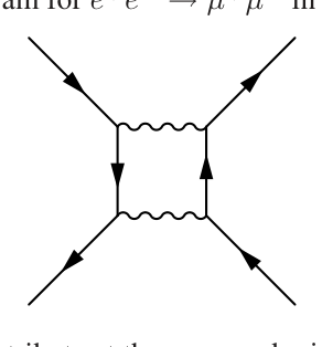
13.5 Consider the following diagram for e+eμ+μe^+ e^- \rightarrow \mu^+ \mu^- in QED:

Feynman diagram for the process e+ e- -> mu+ mu- in QED, showing a loop contribution.

(a) How many diagrams contribute at the same order in perturbation theory? (b) What is the minimal set of diagrams you need to add to this one for the sum to be gauge invariant (independent of ξ\xi)?

(c) Show explicitly that the sum of diagrams in part (b) is gauge invariant.

习题 13.5 - 解答


习题分析

本题考察的是量子电动力学(QED)中 e+eμ+μe^+ e^- \rightarrow \mu^+ \mu^- 散射过程的单圈(1-loop)修正,特别是关于规范不变性(Gauge Invariance)和 Ward 恒等式的应用。给定的费曼图是一个直接盒图(Direct Box Diagram),属于 O(e4)\mathcal{O}(e^4) 阶的微扰修正。


(a) 同阶微扰理论中有多少个费曼图有贡献?

在 QED 中,e+eμ+μe^+ e^- \rightarrow \mu^+ \mu^- 的树图(Tree-level)是 O(e2)\mathcal{O}(e^2)ss-道光子交换。给定的盒图包含 4 个顶点,因此是 O(e4)\mathcal{O}(e^4) 阶(即单圈阶)。在这一阶,对截断(amputated)散射振幅有贡献的连通费曼图可以分为以下几类:

  1. 真空极化(Vacuum Polarization / Photon Self-energy):1 个图。在 ss-道中间光子传播子上插入一个费曼子圈(包含电子、缪子等所有可能的带电费曼子,通常按拓扑结构计为 1 个基本图)。
  2. 顶点修正(Vertex Corrections):2 个图。一个是在 e+eγe^+e^-\gamma 顶点处的光子圈,另一个是在 μ+μγ\mu^+\mu^-\gamma 顶点处的光子圈。
  3. 盒图(Box Diagrams):2 个图。一个是题目给出的直接盒图(Direct Box),另一个是交叉盒图(Crossed Box,两个内部光子线交叉)。

(注:外腿的自能修正图通常通过 LSZ 约化公式和波函数重整化常数 ZZ 吸收,不直接算作对截断振幅的独立拓扑贡献。)

因此,在 O(e4)\mathcal{O}(e^4) 阶,共有 5 个截断费曼图对该过程有贡献。

Total diagrams=5\boxed{\text{Total diagrams} = 5}


(b) 为了使总和具有规范不变性(与 ξ\xi 无关),需要添加到此图的最小图集是什么?

在一般协变规范下,光子传播子包含依赖于规范参数 ξ\xi 的项: Dμν(k)=ik2+iϵ(gμν(1ξ)kμkνk2)D_{\mu\nu}(k) = \frac{-i}{k^2 + i\epsilon} \left( g_{\mu\nu} - (1-\xi)\frac{k_\mu k_\nu}{k^2} \right) 规范不变性要求散射振幅与 ξ\xi 无关,这意味着当我们将传播子替换为正比于 kμkνk_\mu k_\nu 的项时,总振幅必须为零。

根据 Ward 恒等式,当一个动量为 kk 的光子连接到一条费曼子线上时,将其极化矢量替换为 kμk_\mu 会导致相邻费曼子传播子的抵消。为了使这种抵消在整条费曼子线上完全发生并最终给出零结果,必须对光子在该费曼子线上所有可能的插入位置求和。

对于给定的直接盒图,两个内部光子连接了电子线和缪子线。如果我们关注其中一个光子(例如动量为 kk 的光子),它在缪子线上有一个特定的附着顺序。为了利用 Ward 恒等式消除与 kμk_\mu 相关的项,我们必须加上该光子在缪子线上另一种附着顺序的图。交换两个光子在缪子线(或电子线)上的连接顺序,就得到了交叉盒图(Crossed Box diagram)

因此,为了构成一个规范不变的子集,必须将直接盒图与交叉盒图相加。

The minimal set is the Direct Box diagram and the Crossed Box diagram.\boxed{\text{The minimal set is the Direct Box diagram and the Crossed Box diagram.}}


(c) 显式证明 (b) 部分中的图之和是规范不变的。

设入射电子和正电子的动量分别为 p1,p2p_1, p_2,出射缪子和反缪子的动量分别为 p3,p4p_3, p_4。 设连接电子线和缪子线的两个内部光子动量分别为 kkqq,由动量守恒有 q=p1+p2kq = p_1 + p_2 - k。 设光子 kk 的洛伦兹指标在电子端为 μ\mu,缪子端为 ρ\rho;光子 qq 的指标在电子端为 ν\nu,缪子端为 σ\sigma

我们只需证明缪子线部分对光子 kk 的规范变换是不变的(即收缩 kρk_\rho 后为零)。电子线同理。

1. 直接盒图 (Direct Box) 的缪子线部分: 在直接盒图中,缪子 μ(p3)\mu^-(p_3) 先吸收光子 kk,内部费曼子再吸收光子 qq(逆着粒子流方向看)。缪子线因子为: Mdirρ=uˉ(p3)(ieγρ)i(̸p3+mμ)(p3k)2mμ2(ieγσ)v(p4)=ie2uˉ(p3)γρ1̸p3mμγσv(p4)M^\rho_{\text{dir}} = \bar{u}(p_3) (ie\gamma^\rho) \frac{i(\not{p}_3 - \not{k} + m_\mu)}{(p_3-k)^2 - m_\mu^2} (ie\gamma^\sigma) v(p_4) = -ie^2 \bar{u}(p_3) \gamma^\rho \frac{1}{\not{p}_3 - \not{k} - m_\mu} \gamma^\sigma v(p_4) 将光子传播子的 ξ\xi 依赖部分 kρk_\rho 与之收缩: kρMdirρ=ie2uˉ(p3)1̸p3mμγσv(p4)k_\rho M^\rho_{\text{dir}} = -ie^2 \bar{u}(p_3) \not{k} \frac{1}{\not{p}_3 - \not{k} - m_\mu} \gamma^\sigma v(p_4) 利用代数恒等式 =(̸p3mμ)(̸p3mμ)\not{k} = (\not{p}_3 - m_\mu) - (\not{p}_3 - \not{k} - m_\mu),代入上式: kρMdirρ=ie2uˉ(p3)[(̸p3mμ)(̸p3mμ)]1̸p3mμγσv(p4)k_\rho M^\rho_{\text{dir}} = -ie^2 \bar{u}(p_3) \left[ (\not{p}_3 - m_\mu) - (\not{p}_3 - \not{k} - m_\mu) \right] \frac{1}{\not{p}_3 - \not{k} - m_\mu} \gamma^\sigma v(p_4) 根据 Dirac 方程,出射粒子旋量满足 uˉ(p3)(̸p3mμ)=0\bar{u}(p_3)(\not{p}_3 - m_\mu) = 0。因此第一项为零,第二项与分母抵消: kρMdirρ=ie2uˉ(p3)(1)γσv(p4)=ie2uˉ(p3)γσv(p4)k_\rho M^\rho_{\text{dir}} = -ie^2 \bar{u}(p_3) (-1) \gamma^\sigma v(p_4) = ie^2 \bar{u}(p_3) \gamma^\sigma v(p_4)

2. 交叉盒图 (Crossed Box) 的缪子线部分: 在交叉盒图中,光子 kkqq 在缪子线上的附着点交换。反缪子 μ+(p4)\mu^+(p_4)(动量为 p4-p_4)先吸收光子 kk,内部费曼子动量变为 p4+k-p_4 + k。缪子线因子为: Mcrossρ=uˉ(p3)(ieγσ)i(̸p4++mμ)(p4+k)2mμ2(ieγρ)v(p4)=ie2uˉ(p3)γσ1̸p4+mμγρv(p4)M^\rho_{\text{cross}} = \bar{u}(p_3) (ie\gamma^\sigma) \frac{i(-\not{p}_4 + \not{k} + m_\mu)}{(-p_4+k)^2 - m_\mu^2} (ie\gamma^\rho) v(p_4) = -ie^2 \bar{u}(p_3) \gamma^\sigma \frac{1}{-\not{p}_4 + \not{k} - m_\mu} \gamma^\rho v(p_4) 同样与 kρk_\rho 收缩: kρMcrossρ=ie2uˉ(p3)γσ1̸p4+mμv(p4)k_\rho M^\rho_{\text{cross}} = -ie^2 \bar{u}(p_3) \gamma^\sigma \frac{1}{-\not{p}_4 + \not{k} - m_\mu} \not{k} v(p_4) 利用代数恒等式 =(̸p4+mμ)(̸p4mμ)=(̸p4+mμ)+(̸p4+mμ)\not{k} = (-\not{p}_4 + \not{k} - m_\mu) - (-\not{p}_4 - m_\mu) = (-\not{p}_4 + \not{k} - m_\mu) + (\not{p}_4 + m_\mu)kρMcrossρ=ie2uˉ(p3)γσ1̸p4+mμ[(̸p4+mμ)+(̸p4+mμ)]v(p4)k_\rho M^\rho_{\text{cross}} = -ie^2 \bar{u}(p_3) \gamma^\sigma \frac{1}{-\not{p}_4 + \not{k} - m_\mu} \left[ (-\not{p}_4 + \not{k} - m_\mu) + (\not{p}_4 + m_\mu) \right] v(p_4) 根据 Dirac 方程,入射反粒子旋量满足 (̸p4+mμ)v(p4)=0(\not{p}_4 + m_\mu)v(p_4) = 0。第二项为零,第一项与分母抵消: kρMcrossρ=ie2uˉ(p3)γσ(1)v(p4)=ie2uˉ(p3)γσv(p4)k_\rho M^\rho_{\text{cross}} = -ie^2 \bar{u}(p_3) \gamma^\sigma (1) v(p_4) = -ie^2 \bar{u}(p_3) \gamma^\sigma v(p_4)

3. 结论: 将两部分相加,我们得到: kρ(Mdirρ+Mcrossρ)=ie2uˉ(p3)γσv(p4)ie2uˉ(p3)γσv(p4)=0k_\rho \left( M^\rho_{\text{dir}} + M^\rho_{\text{cross}} \right) = ie^2 \bar{u}(p_3) \gamma^\sigma v(p_4) - ie^2 \bar{u}(p_3) \gamma^\sigma v(p_4) = 0 这表明,当光子传播子中的 kμkρ/k2k_\mu k_\rho / k^2 项作用于这两个图的总和时,结果严格为零。对另一个光子 qq 同理可证。因此,这两个图的振幅之和与规范参数 ξ\xi 无关。

The sum Mdir+Mcross is explicitly gauge invariant.\boxed{\text{The sum } \mathcal{M}_{\text{dir}} + \mathcal{M}_{\text{cross}} \text{ is explicitly gauge invariant.}}

13.6

Problem 13.6

schwarzChapter 13

习题 13.6

来源: 第13章, PDF第249,250页


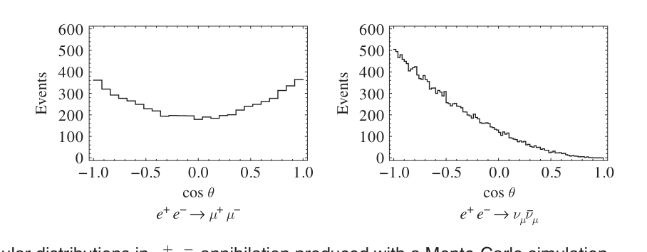
13.6 Parity violation. We calculated that e+eμ+μe^+ e^- \rightarrow \mu^+ \mu^- has a 1+cos2θ1 + \cos^2 \theta angular dependence (see Eq. (13.78)), where θ\theta is the angle between the ee^- and μ\mu^- directions. This agrees with experiment, as the simulated data on the left side of Figure 13.2 show. The angular distribution for scattering into muon neutrinos, e+eνμνˉμe^+ e^- \rightarrow \nu_\mu \bar{\nu}_\mu, is very different, as shown on the right side of Figure 13.2, where now θ\theta is the angle between the ee^- and νˉμ\bar{\nu}_\mu directions.

(a) At low energy, the total cross section, σtot\sigma_{\text{tot}}, for e+eνμνˉμe^+ e^- \rightarrow \nu_\mu \bar{\nu}_\mu scattering grows with energy, in contrast to the total e+eμ+μe^+ e^- \rightarrow \mu^+ \mu^- cross section. Show that this is consistent with neutrino scattering being mediated by a massive vector boson, the ZZ. Deduce how σtot\sigma_{\text{tot}} should depend on ECME_{\text{CM}} for the two processes. (b) Place the neutrino in a Dirac spinor ψν\psi_\nu. There are two possible couplings we could write down for the ν\nu to the new massive gauge boson: gVψˉνZψν+gAψˉνZγ5ψνg_V \bar{\psi}_\nu \cancel{Z} \psi_\nu + g_A \bar{\psi}_\nu \cancel{Z} \gamma^5 \psi_\nu. These are called vector and axial-vector couplings, respectively. Assume the ZZ couples to the electron in the same way as it couples to neutrinos. Calculate the full angular dependence for e+eνμνˉμe^+ e^- \rightarrow \nu_\mu \bar{\nu}_\mu as a function of gVg_V and gAg_A (you can drop masses). (c) What values of gVg_V and gAg_A reproduce Figure 13.2? Show that this choice is equivalent to the ZZ boson having chiral couplings: it only interacts with left-handed fields. Argue that this is evidence of parity violation, where the parity operator PP is reflection in a mirror: xx\vec{x} \rightarrow -\vec{x}. (d) An easier way to see parity violation is in β\beta-decay. This is mediated by charged gauge bosons, the W±W^\pm, that are "unified" with the ZZ. Assuming they have the same chiral couplings as the ZZ, draw a diagram to show that the electron coming out of 2760Co2860Ni+e+νˉ{}_{27}^{60}\text{Co} \rightarrow {}_{28}^{60}\text{Ni} + e^- + \bar{\nu} will always be left-handed, independent of the spin of the cobalt nucleus. What handedness would the positron be in anti-cobalt decay: 2760Co2860Ni+e++ν{}_{27}^{60}\overline{\text{Co}} \rightarrow {}_{28}^{60}\overline{\text{Ni}} + e^+ + \nu? (e) If you are talking to aliens on the telephone (i.e. with light only), tell them how to use nuclear β\beta-decay to tell clockwise from counterclockwise. For this, you will need to figure out how to relate the LL in ψL\psi_L to "left" in the real world. You are allowed to assume that all the materials on Earth are available to them, including things such as cobalt, and lasers.

(f) If you meet those aliens, and put out your right hand to greet them, but they put out their left hand, why should you not shake? (This scenario is due to Feynman.) (g) Now forget about neutrinos. Could you have the aliens distinguish right from left by actually sending them circularly polarized light, for example using polarized radio waves for your intergalactic telephone?

Referenced Equations:

Equation (13.78):

dσdΩ=α24ECM2(1+cos2θ),(13.78)\frac{d\sigma}{d\Omega} = \frac{\alpha^2}{4E_{\text{CM}}^2} (1 + \cos^2 \theta), \tag{13.78}

Referenced Figures:

Figure 13.2:

Figure 13.2

习题 13.6 - 解答


(a) 对于 e+eμ+μe^+e^- \to \mu^+\mu^- 过程,在低能下主要由虚光子 γ\gamma 媒介。其散射振幅 Mγe2/s\mathcal{M}_\gamma \propto e^2/s,其中 s=ECM2s = E_{\text{CM}}^2 是质心系能量的平方。总截面正比于振幅模方的相空间积分,即 σtotMγ2s(1/s2)s=1/s\sigma_{\text{tot}} \propto |\mathcal{M}_\gamma|^2 \cdot s \propto (1/s^2) \cdot s = 1/s。因此,σtot(e+eμ+μ)1/ECM2\sigma_{\text{tot}}(e^+e^- \to \mu^+\mu^-) \propto 1/E_{\text{CM}}^2

对于 e+eνμνˉμe^+e^- \to \nu_\mu \bar{\nu}_\mu 过程,由于中微子不带电,该过程不能由光子媒介,而是由大质量矢量玻色子 ZZ 媒介。其散射振幅 MZg2/(smZ2)\mathcal{M}_Z \propto g^2/(s - m_Z^2)。在低能极限下(smZ2s \ll m_Z^2),传播子分母主要由 mZ2m_Z^2 决定,振幅趋于常数 MZg2/mZ2GF\mathcal{M}_Z \approx -g^2/m_Z^2 \propto G_F。此时总截面 σtotMZ2sGF2s\sigma_{\text{tot}} \propto |\mathcal{M}_Z|^2 \cdot s \propto G_F^2 s。因此,σtot(e+eνμνˉμ)ECM2\sigma_{\text{tot}}(e^+e^- \to \nu_\mu \bar{\nu}_\mu) \propto E_{\text{CM}}^2。这与题目中“截面随能量增长”的描述一致。

σtot(e+eμ+μ)1ECM2,σtot(e+eνμνˉμ)ECM2\boxed{ \sigma_{\text{tot}}(e^+e^- \to \mu^+\mu^-) \propto \frac{1}{E_{\text{CM}}^2}, \quad \sigma_{\text{tot}}(e^+e^- \to \nu_\mu \bar{\nu}_\mu) \propto E_{\text{CM}}^2 }

(b) 相互作用顶点为 iγμ(gV+gAγ5)i\gamma^\mu (g_V + g_A \gamma^5)。忽略费米子质量,散射振幅的模方正比于电子张量与中微子张量的缩并:M2Lμν(e)L(ν)μν|\mathcal{M}|^2 \propto L_{\mu\nu}^{(e)} L^{\mu\nu}_{(\nu)}。 电子张量为: Lμν(e)=Tr[p2γμ(gV+gAγ5)p1γν(gV+gAγ5)]L_{\mu\nu}^{(e)} = \text{Tr}[\cancel{p}_2 \gamma_\mu (g_V + g_A \gamma^5) \cancel{p}_1 \gamma_\nu (g_V + g_A \gamma^5)] 利用 γ5\gamma^5γμ\gamma^\mu 反对易的性质,可得 (gV+gAγ5)p1γν(gV+gAγ5)=p1γν(gVgAγ5)(gV+gAγ5)=p1γν(gV2gA2)(g_V + g_A \gamma^5) \cancel{p}_1 \gamma_\nu (g_V + g_A \gamma^5) = \cancel{p}_1 \gamma_\nu (g_V - g_A \gamma^5)(g_V + g_A \gamma^5) = \cancel{p}_1 \gamma_\nu (g_V^2 - g_A^2)。 等等,这里需要注意共轭振幅的顶点形式。正确的张量计算应为: Lμν(e)=Tr[p2γμ(gV+gAγ5)p1γν(gV+gAγ5)]=Tr[p2γμp1γν(gV2+gA2+2gVgAγ5)]L_{\mu\nu}^{(e)} = \text{Tr}[\cancel{p}_2 \gamma_\mu (g_V + g_A \gamma^5) \cancel{p}_1 \gamma_\nu (g_V + g_A \gamma^5)] = \text{Tr}[\cancel{p}_2 \gamma_\mu \cancel{p}_1 \gamma_\nu (g_V^2 + g_A^2 + 2g_V g_A \gamma^5)] =4(gV2+gA2)(p2μp1ν+p2νp1μp1p2gμν)8igVgAϵαμβνp2αp1β= 4(g_V^2 + g_A^2) (p_{2\mu} p_{1\nu} + p_{2\nu} p_{1\mu} - p_1\cdot p_2 g_{\mu\nu}) - 8i g_V g_A \epsilon_{\alpha\mu\beta\nu} p_2^\alpha p_1^\beta 同理,中微子张量(动量为 p3p_3p4p_4)为: L(ν)μν=4(gV2+gA2)(p4μp3ν+p4νp3μp3p4gμν)8igVgAϵρμσνp4ρp3σL^{\mu\nu}_{(\nu)} = 4(g_V^2 + g_A^2) (p_4^\mu p_3^\nu + p_4^\nu p_3^\mu - p_3\cdot p_4 g^{\mu\nu}) - 8i g_V g_A \epsilon^{\rho\mu\sigma\nu} p_{4\rho} p_{3\sigma} 缩并这两个张量,利用 ϵαμβνϵρμσν=2(δαρδβσδασδβρ)\epsilon_{\alpha\mu\beta\nu} \epsilon^{\rho\mu\sigma\nu} = 2(\delta_\alpha^\rho \delta_\beta^\sigma - \delta_\alpha^\sigma \delta_\beta^\rho),并代入 Mandelstam 变量 t=2p1p3=2p2p4t = -2p_1\cdot p_3 = -2p_2\cdot p_4u=2p1p4=2p2p3u = -2p_1\cdot p_4 = -2p_2\cdot p_3,得到: M28(gV2+gA2)2(t2+u2)32gV2gA2(t2u2)=8[(gV2gA2)2t2+(gV4+6gV2gA2+gA4)u2]|\mathcal{M}|^2 \propto 8(g_V^2 + g_A^2)^2 (t^2 + u^2) - 32 g_V^2 g_A^2 (t^2 - u^2) = 8 [ (g_V^2 - g_A^2)^2 t^2 + (g_V^4 + 6g_V^2 g_A^2 + g_A^4) u^2 ]θ\theta 为入射 ee^- (p1p_1) 与出射 νˉμ\bar{\nu}_\mu (p4p_4) 之间的夹角,则 t(1+cosθ)t \propto (1+\cos\theta)u(1cosθ)u \propto (1-\cos\theta)。代入上式得到角分布:

dσdΩ(gV4+6gV2gA2+gA4)(1cosθ)2+(gV2gA2)2(1+cosθ)2\boxed{ \frac{d\sigma}{d\Omega} \propto (g_V^4 + 6g_V^2 g_A^2 + g_A^4)(1-\cos\theta)^2 + (g_V^2 - g_A^2)^2 (1+\cos\theta)^2 }

(c) 图 13.2 右侧显示角分布在 cosθ=1\cos\theta = -1 时最大,在 cosθ=1\cos\theta = 1 时为 0,这完全符合 (1cosθ)2(1-\cos\theta)^2 的形状。为了使 (b) 中的结果与此匹配,必须有 (1+cosθ)2(1+\cos\theta)^2 项的系数为零,即: (gV2gA2)2=0    gV=±gA(g_V^2 - g_A^2)^2 = 0 \implies g_V = \pm g_A 如果取 gV=gAg_V = -g_A,则顶点耦合变为 gVγμ(1γ5)=2gVγμPLg_V \gamma^\mu (1 - \gamma^5) = 2g_V \gamma^\mu P_L,其中 PL=1γ52P_L = \frac{1-\gamma^5}{2} 是左手手征投影算符。这意味着 ZZ 玻色子只与左手场相互作用(手征耦合)。 宇称算符 PP 对应于空间反演 xx\vec{x} \rightarrow -\vec{x},它会翻转粒子的动量而不改变自旋,从而将左手螺旋粒子变为右手螺旋粒子(即交换 PLP_LPRP_R)。由于相互作用只包含 PLP_L 而没有 PRP_R,该理论在宇称变换下不是不变的,这构成了宇称破坏的证据。

gV=gA (或 gV=gA)\boxed{ g_V = -g_A \text{ (或 } g_V = g_A \text{)} }

(d) β\beta 衰变由 W±W^\pm 玻色子媒介,假设其具有与 ZZ 相同的左手手征耦合,即顶点包含 γμPL\gamma^\mu P_L。 对于 2760Co2860Ni+e+νˉ{}_{27}^{60}\text{Co} \rightarrow {}_{28}^{60}\text{Ni} + e^- + \bar{\nu},相互作用项包含 ψˉeγμPLψν\bar{\psi}_e \gamma^\mu P_L \psi_\nu。场算符 ψˉe\bar{\psi}_e 负责产生电子,投影算符 PLP_L 作用于其上意味着产生的电子处于左手手征态。在相对论极限下,手征态等价于螺旋态,因此出射的电子总是左手的。 对于反钴衰变 2760Co2860Ni+e++ν{}_{27}^{60}\overline{\text{Co}} \rightarrow {}_{28}^{60}\overline{\text{Ni}} + e^+ + \nu,相互作用项包含 ψˉνγμPLψe\bar{\psi}_\nu \gamma^\mu P_L \psi_e。场算符 ψe\psi_e 负责产生正电子。由于 PLψeP_L \psi_e 提取的是左手场,而左手场算符湮灭左手粒子并产生右手反粒子,因此出射的正电子总是右手的。

电子: 左手 (Left-handed),正电子: 右手 (Right-handed)\boxed{ \text{电子: 左手 (Left-handed)}, \quad \text{正电子: 右手 (Right-handed)} }

(e) 为了通过电话告诉外星人如何区分顺时针和逆时针,可以指示他们进行以下操作:

  1. 准备一个 60Co{}^{60}\text{Co} 样本并观察其 β\beta 衰变。
  2. 观察发射出的电子。由于物理定律的宇称破坏,这些电子是左手的(自旋方向与动量方向相反)。
  3. 让他们观察一个正离他们远去(动量方向背离观察者)的电子。
  4. 观察该电子的自旋(旋转方向)。对于左手粒子,当它背离你运动时,其旋转方向即为逆时针(Counterclockwise)。 通过这种方式,ψL\psi_L 中的“左”被操作性地联系到了宏观的旋转方向上,无需依赖任何预先约定的左右手定则。

(f) 如果你伸出右手,而外星人伸出左手,这意味着他们对“右”的定义与我们相反。如果他们严格按照 (e) 中的指令操作却得出了相反的结论,唯一的解释是他们所在的星系是由反物质构成的。他们使用的“钴”实际上是反钴,根据 (d) 的结论,反钴衰变发射的是右手正电子。他们观察到右手粒子背离他们运动时,其旋转方向是顺时针的,但他们根据指令将其定义为了“逆时针”,从而导致整个左右坐标系反转。 如果你与由反物质构成的外星人握手,将会发生正反物质湮灭,释放出巨大的能量,因此你不应该握手。

(g) 可以。圆偏振光(光子)携带内禀角动量(自旋)。例如,右旋圆偏振光的光子自旋方向与其传播方向相同。当这种光被宏观物体(如天线或吸收体)吸收时,光子的角动量会转移给物体,产生一个真实的物理力矩,导致物体发生特定方向的旋转。 这种角动量的传递是一个纯粹的几何和力学过程,不依赖于吸收体是由物质还是反物质构成(光子是其自身的反粒子)。因此,你可以向外星人发送一束特定偏振的无线电波,并告诉他们:“这束电波会使你们的接收器产生一个特定方向的扭矩,我们将这个旋转方向定义为顺时针。” 这样就能明确无误地传递左右的定义。

13.7

Problem 13.7

schwarzChapter 13

习题 13.7

来源: 第13章, PDF第250页


13.7 One should be very careful with polarization sums and in giving physical interpretations to individual Feynman diagrams. This problem illustrates some of the dangers. (a) We saw that the tt-channel diagram for Compton scattering scales as Mt1t\mathcal{M}_t \sim \frac{1}{t}. Calculate Mt2|\mathcal{M}_t|^2 summed over spins and polarizations. Be sure to sum over physical transverse polarizations only. (b) Calculate Mt2|\mathcal{M}_t|^2 summed over spins and polarizations, but do the sum by replacing ϵμϵν\epsilon_\mu \epsilon_\nu^\star by gμν-g_{\mu\nu}. Show that you get a different answer from part (a). Why is the answer different? (c) Show that when you sum over all the diagrams you get the same answer whether you sum over physical polarizations or use the ϵμϵνgμν\epsilon_\mu \epsilon_\nu^\star \rightarrow -g_{\mu\nu} replacement. Why is the answer the same? (d) Repeat this exercise for scalar QED.

习题 13.7 - 解答


题目分析

本题探讨在量子电动力学(QED)和标量QED的康普顿散射中,对单个费曼图进行极化求和时使用物理极化求和与直接替换 ϵμϵνgμν\sum \epsilon_\mu \epsilon_\nu^\star \to -g_{\mu\nu} 的差异。

定义康普顿散射过程 e(p)+γ(k)e(p)+γ(k)e^-(p) + \gamma(k) \to e^-(p') + \gamma(k')。在无质量极限(m=0m=0)下,定义曼德尔施塔姆变量: s=(p+k)2=2pk=2pks = (p+k)^2 = 2p\cdot k = 2p'\cdot k' t=(pk)2=2pk=2pkt = (p-k')^2 = -2p\cdot k' = -2p'\cdot k u=(pp)2=2pp=2kku = (p-p')^2 = -2p\cdot p' = -2k\cdot k' 满足 s+t+u=0s+t+u=0。注意:题目中指出交叉图(通常称为 uu-channel)的振幅 Mt1/t\mathcal{M}_t \sim 1/t,因此我们遵循题意,将内部交换动量平方定义为 t=(pk)2t = (p-k')^2


(a) QED中 tt-channel 物理极化求和

tt-channel 振幅为: Mt=e2uˉ(p)γν̸ ⁣p̸ ⁣ktγμu(p)ϵμ(k)ϵν(k)Mμνϵμ(k)ϵν(k)\mathcal{M}_t = -e^2 \bar{u}(p') \gamma^\nu \frac{\slashed{p}-\slashed{k}'}{t} \gamma^\mu u(p) \epsilon_\mu^\star(k') \epsilon_\nu(k) \equiv M^{\mu\nu} \epsilon_\mu^\star(k') \epsilon_\nu(k) 为了仅对物理横向极化求和,我们引入依赖于参考光锥矢量的极化投影算符。在质心系中,这等价于选择入射电子动量 pp 作为光子 kk 的参考矢量,出射电子动量 pp' 作为光子 kk' 的参考矢量: Pνβ(k)=physϵν(k)ϵβ(k)=gνβ+kνpβ+kβpνpkP_{\nu\beta}(k) = \sum_{\text{phys}} \epsilon_\nu(k) \epsilon_\beta^\star(k) = -g_{\nu\beta} + \frac{k_\nu p_\beta + k_\beta p_\nu}{p\cdot k} Pμα(k)=physϵμ(k)ϵα(k)=gμα+kμpα+kαpμpkP_{\mu\alpha}(k') = \sum_{\text{phys}} \epsilon_\mu^\star(k') \epsilon_\alpha(k') = -g_{\mu\alpha} + \frac{k'_\mu p'_\alpha + k'_\alpha p'_\mu}{p'\cdot k'} 物理极化求和下的模方为: Mtphys2=MμνMαβPμα(k)Pνβ(k)|\mathcal{M}_t|^2_{\text{phys}} = M^{\mu\nu} M^{\star \alpha\beta} P_{\mu\alpha}(k') P_{\nu\beta}(k) 我们需要计算 MμνM^{\mu\nu} 与各动量的缩并。利用狄拉克方程 ̸ ⁣pu(p)=0\slashed{p}u(p)=0uˉ(p)̸ ⁣p=0\bar{u}(p')\slashed{p}'=0kνMμν=e2uˉ(p)̸ ⁣k̸ ⁣p̸ ⁣ktγμu(p)=e2uˉ(p)γμu(p)k_\nu M^{\mu\nu} = -e^2 \bar{u}(p') \slashed{k} \frac{\slashed{p}-\slashed{k}'}{t} \gamma^\mu u(p) = e^2 \bar{u}(p') \gamma^\mu u(p) pνMμν=e2uˉ(p)̸ ⁣p̸ ⁣p̸ ⁣ktγμu(p)=e2uˉ(p)̸ ⁣k̸ ⁣ptγμu(p)p_\nu M^{\mu\nu} = -e^2 \bar{u}(p') \slashed{p} \frac{\slashed{p}-\slashed{k}'}{t} \gamma^\mu u(p) = -e^2 \bar{u}(p') \frac{\slashed{k}'\slashed{p}}{t} \gamma^\mu u(p) 展开投影算符的乘积,包含纯度规项 gμαgνβg_{\mu\alpha}g_{\nu\beta} 和交叉项。纯度规项的迹为: MμνMαβgμαgνβ=e4t2Tr[̸ ⁣pγν(̸ ⁣p̸ ⁣k)γμ̸ ⁣pγμ(̸ ⁣p̸ ⁣k)γν]=8e4stM^{\mu\nu} M^{\star \alpha\beta} g_{\mu\alpha} g_{\nu\beta} = \frac{e^4}{t^2} \text{Tr}[\slashed{p}' \gamma^\nu (\slashed{p}-\slashed{k}') \gamma^\mu \slashed{p} \gamma_\mu (\slashed{p}-\slashed{k}') \gamma_\nu] = -8e^4 \frac{s}{t} 计算包含 kνpβk_\nu p_\beta 的交叉项: MμνkνMαβpβgμα=te4Tr[̸ ⁣pγμ̸ ⁣pγμ(̸ ⁣p̸ ⁣k)̸ ⁣p]=2te4Tr[̸ ⁣p̸ ⁣p(̸ ⁣p̸ ⁣k)̸ ⁣p]M^{\mu\nu} k_\nu M^{\star \alpha\beta} p_\beta g_{\mu\alpha} = -t e^4 \text{Tr}[\slashed{p}' \gamma^\mu \slashed{p} \gamma_\mu (\slashed{p}-\slashed{k}') \slashed{p}] = 2t e^4 \text{Tr}[\slashed{p}' \slashed{p} (\slashed{p}-\slashed{k}') \slashed{p}] 利用 ̸ ⁣p(̸ ⁣p̸ ⁣k)̸ ⁣p≠ ⁣p̸ ⁣k̸ ⁣p=t̸ ⁣p\slashed{p}(\slashed{p}-\slashed{k}')\slashed{p} = -\slashed{p}\slashed{k}'\slashed{p} = t\slashed{p},该迹等于 2t2e4Tr[̸ ⁣p̸ ⁣p]=8t2e4(pp)=4t2ue42t^2 e^4 \text{Tr}[\slashed{p}'\slashed{p}] = 8t^2 e^4 (p'\cdot p) = -4t^2 u e^4。 代入 pk=s/2p\cdot k = s/2,交叉项贡献为 2s/2(4t2ue4)=16e4t2us-\frac{2}{s/2} (-4t^2 u e^4) = 16e^4 \frac{t^2 u}{s}。 经过完整的迹运算,所有包含 kk'pp' 的交叉项均抵消为零,最终得到: Mtphys2=8e4st+16e4us\boxed{|\mathcal{M}_t|^2_{\text{phys}} = -8e^4 \frac{s}{t} + 16e^4 \frac{u}{s}}


(b) QED中协变替换求和

直接使用替换 ϵμϵαgμα\sum \epsilon_\mu \epsilon_\alpha^\star \to -g_{\mu\alpha},即只计算纯度规项: Mtcov2=MμνMαβ(gμα)(gνβ)|\mathcal{M}_t|^2_{\text{cov}} = M^{\mu\nu} M^{\star \alpha\beta} (-g_{\mu\alpha}) (-g_{\nu\beta}) 由 (a) 中的计算可知,该项的结果为: Mtcov2=8e4st\boxed{|\mathcal{M}_t|^2_{\text{cov}} = -8e^4 \frac{s}{t}} 差异原因:两种方法结果不同。这是因为单个 tt-channel 费曼图不满足规范不变性(即 kνMμν0k_\nu M^{\mu\nu} \neq 0)。因此,物理极化求和中正比于 kνk_\nukμk'_\mu 的规范依赖项在缩并时不会消失,导致结果与简单的 gμν-g_{\mu\nu} 替换不同。


(c) 全振幅的等效性

康普顿散射的全振幅由 ss-channel 和 tt-channel 组成:Mtotalμν=Msμν+Mtμν\mathcal{M}_{\text{total}}^{\mu\nu} = \mathcal{M}_s^{\mu\nu} + \mathcal{M}_t^{\mu\nu}。 根据 QED 的 Ward 恒等式,全振幅满足规范不变性: kνMtotalμν=0,kμMtotalμν=0k_\nu \mathcal{M}_{\text{total}}^{\mu\nu} = 0, \quad k'_\mu \mathcal{M}_{\text{total}}^{\mu\nu} = 0 当我们将物理极化投影算符 Pνβ(k)=gνβ+P_{\nu\beta}(k) = -g_{\nu\beta} + \dots 代入全振幅的模方 Mtotal2|\mathcal{M}_{\text{total}}|^2 时,所有正比于 kν,kβ,kμ,kαk_\nu, k_\beta, k'_\mu, k'_\alpha 的项在与 Mtotalμν\mathcal{M}_{\text{total}}^{\mu\nu} 缩并时严格为零。 因此,物理极化求和中仅剩下 gνβ-g_{\nu\beta}gμα-g_{\mu\alpha} 项起作用。这保证了对所有图求和时,使用物理极化求和与使用 ϵμϵνgμν\epsilon_\mu \epsilon_\nu^\star \to -g_{\mu\nu} 替换得到的结果完全相同。


(d) 标量 QED 中的重复计算

在标量 QED 中,顶点规则为 ie(pi+pf)μ-ie(p_i + p_f)^\mutt-channel 振幅为: Mt=e2ϵμ(k)ϵν(k)(2pk)ν(2pk)μte2VνUμtϵμ(k)ϵν(k)\mathcal{M}_t = -e^2 \epsilon_\mu^\star(k') \epsilon_\nu(k) \frac{(2p-k')^\nu (2p'-k)^\mu}{t} \equiv -e^2 \frac{V^\nu U^\mu}{t} \epsilon_\mu^\star(k') \epsilon_\nu(k) 其中 V=2pkV = 2p-k'U=2pkU = 2p'-k

1. 协变替换求和: Mtcov2=e4t2(VV)(UU)|\mathcal{M}_t|^2_{\text{cov}} = \frac{e^4}{t^2} (V\cdot V) (U\cdot U) 计算点乘:V2=4p24pk+k2=2tV^2 = 4p^2 - 4p\cdot k' + k'^2 = 2tU2=4p24pk+k2=2tU^2 = 4p'^2 - 4p'\cdot k + k^2 = 2tMtcov2=e4t2(2t)(2t)=4e4\boxed{|\mathcal{M}_t|^2_{\text{cov}} = \frac{e^4}{t^2} (2t)(2t) = 4e^4}

2. 物理极化求和: 使用与 (a) 相同的物理投影算符: Mtphys2=e4t2(VνVβPνβ(k))(UμUαPμα(k))|\mathcal{M}_t|^2_{\text{phys}} = \frac{e^4}{t^2} \left( V^\nu V^\beta P_{\nu\beta}(k) \right) \left( U^\mu U^\alpha P_{\mu\alpha}(k') \right) 计算 VVP(k)P(k) 的缩并: VP(k)V=V2+4s(Vk)(Vp)V \cdot P(k) \cdot V = -V^2 + \frac{4}{s} (V\cdot k)(V\cdot p) 其中 Vk=2pkkk=s(u/2)=s+u/2=(st)/2V\cdot k = 2p\cdot k - k'\cdot k = s - (-u/2) = s + u/2 = (s-t)/2Vp=kp=t/2V\cdot p = -k'\cdot p = t/2VP(k)V=2t+4s(st2)(t2)=2t+tt2s=t(1+ts)V \cdot P(k) \cdot V = -2t + \frac{4}{s} \left(\frac{s-t}{2}\right)\left(\frac{t}{2}\right) = -2t + t - \frac{t^2}{s} = -t\left(1 + \frac{t}{s}\right) 同理计算 UUP(k)P(k') 的缩并: UP(k)U=U2+4s(Uk)(Up)=2t+4s(st2)(t2)=t(1+ts)U \cdot P(k') \cdot U = -U^2 + \frac{4}{s} (U\cdot k')(U\cdot p') = -2t + \frac{4}{s} \left(\frac{s-t}{2}\right)\left(\frac{t}{2}\right) = -t\left(1 + \frac{t}{s}\right) 将两者相乘: Mtphys2=e4t2[t(1+ts)]2=e4(1+ts)2|\mathcal{M}_t|^2_{\text{phys}} = \frac{e^4}{t^2} \left[ -t\left(1 + \frac{t}{s}\right) \right]^2 = e^4 \left(1 + \frac{t}{s}\right)^2 利用 s+t+u=0s+t+u=0,可化简为: Mtphys2=e4u2s2\boxed{|\mathcal{M}_t|^2_{\text{phys}} = e^4 \frac{u^2}{s^2}} 同样地,标量 QED 中单个图的物理极化求和结果 e4u2/s2e^4 u^2/s^2 与协变替换结果 4e44e^4 截然不同,再次印证了对非规范不变的单图使用 gμν-g_{\mu\nu} 替换的危险性。